
Polynomial Regression
Polynomial regression extends beyond simple linear models, offering a powerful approach to capture curved relationships in your data. Whether you’re a student exploring statistical concepts or a professional seeking to enhance predictive modeling skills, polynomial regression provides essential techniques for modeling complex, non-linear patterns.
What is Polynomial Regression?
Polynomial regression is a form of regression analysis where the relationship between the independent variable X and the dependent variable Y is modeled as an nth degree polynomial. Unlike linear regression that fits a straight line to data, polynomial regression fits a curve by introducing polynomial terms.
The general form of a polynomial regression model can be expressed as:
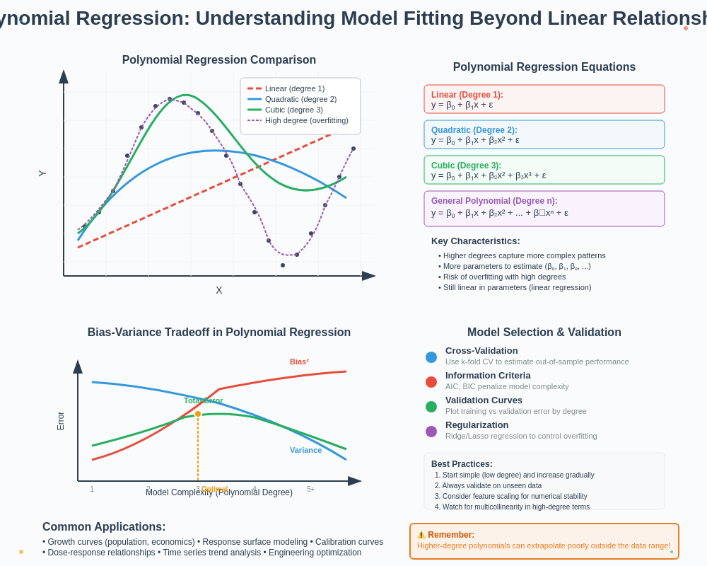
Y = β₀ + β₁X + β₂X² + β₃X³ + … + βₙXⁿ + ε
Where:
- Y is the dependent variable
- X is the independent variable
- β₀, β₁, β₂, … βₙ are the regression coefficients
- ε represents the error term
When to Use Polynomial Regression
Polynomial regression becomes particularly useful when:
- Data shows clear curvature that linear models can’t capture
- Relationships between variables aren’t monotonic
- You need to model peaks and valleys in your data
- Simple linear models show systematic patterns in residuals
Comparing Linear vs. Polynomial Regression
| Feature | Linear Regression | Polynomial Regression |
|---|---|---|
| Equation Form | Y = β₀ + β₁X + ε | Y = β₀ + β₁X + β₂X² + … + βₙXⁿ + ε |
| Curve Type | Straight line | Curved line (parabola, cubic, etc.) |
| Flexibility | Low – fixed slope | High – can model complex relationships |
| Risk of Overfitting | Lower | Higher (especially with higher degrees) |
| Interpretability | High | Decreases with polynomial degree |
| Implementation Complexity | Simpler | More complex |
How to Implement Polynomial Regression
Implementing polynomial regression involves several key steps that transform your data and prepare it for modeling:
1. Feature Transformation
The first step in polynomial regression is creating polynomial features from your original input variables. This process involves raising your original feature to various powers.
For instance, if X is your original feature:
- X¹ remains as is
- X² is the square of the original values
- X³ is the cube of the original values
2. Model Fitting and Estimation
Once you’ve created polynomial features, the actual fitting process is similar to multiple linear regression. The model estimates coefficients that minimize the sum of squared residuals between predicted and actual values.
Tools commonly used for polynomial regression implementation:
- Python: scikit-learn’s
PolynomialFeaturesandLinearRegression - R:
lm()function with polynomial terms - Excel: Trendline options in scatter plots
- SPSS: Curve Estimation procedures
3. Selecting the Optimal Polynomial Degree
One of the most crucial decisions in polynomial regression is selecting the appropriate polynomial degree. This balance is essential for creating a model that generalizes well to new data.
| Degree | Model Behavior | Typical Use Case |
|---|---|---|
| 1 | Linear (straight line) | Simple monotonic relationships |
| 2 | Quadratic (one curve) | Data with a single peak or valley |
| 3 | Cubic (complex curve) | Data with multiple inflection points |
| 4+ | Higher-order curves | Very complex patterns (use with caution) |
Methods for selecting optimal degree:
- Cross-validation
- Information criteria (AIC, BIC)
- Adjusted R-squared analysis
- Visualization of fitted curves
Challenges and Limitations of Polynomial Regression
While polynomial regression offers flexibility, it comes with several important considerations:
- Overfitting: Higher-degree polynomials can capture noise rather than true patterns
- Extrapolation risks: Predictions outside the data range can become wildly inaccurate
- Multicollinearity: High correlation between polynomial terms can cause unstable estimates
- Interpretability: Higher-degree models become harder to interpret meaningfully
Dealing with overfitting:
- Use regularization techniques (Ridge, Lasso)
- Apply cross-validation to test generalization
- Consider alternative non-linear models
Applications of Polynomial Regression
Polynomial regression finds applications across numerous fields:
• Economics: Modeling production functions and economic growth patterns
• Physics: Describing physical laws and trajectories
• Biology: Growth curves and population dynamics
• Engineering: Material stress-strain relationships
• Environmental science: Pollution concentration models
• Finance: Risk assessment and return modeling
Real-World Example: Temperature Variation
Temperature changes throughout the day typically follow a curved pattern rather than a linear one. A polynomial model of degree 2 or 3 can effectively capture the morning rise, midday peak, and evening decline in temperature.
Alternatives to Polynomial Regression
When polynomial regression isn’t ideal, several alternatives are available:
| Method | Strengths | Best Used When |
|---|---|---|
| Splines | Local flexibility, controlled complexity | Data has different behaviors in different regions |
| GAMs | Can model very complex relationships | You need interpretable non-linear effects |
| Decision Trees | Handle non-linear relationships without transformation | Data has hierarchical structure or many features |
| Neural Networks | Extremely flexible, can model complex patterns | Large datasets with complex non-linear relationships |
Evaluating Polynomial Regression Models
Effective evaluation ensures your polynomial regression model provides reliable insights and predictions:
Key Metrics and Visual Tools
• R-squared: Measures proportion of variance explained by the model
• Adjusted R-squared: R-squared adjusted for model complexity
• RMSE (Root Mean Squared Error): Average magnitude of prediction errors
• Residual plots: Visual check for patterns suggesting model inadequacy
• Q-Q plots: Assess normality assumption of residuals
Validation Approaches
- Train-test splits: Reserve portion of data to evaluate model performance
- K-fold cross-validation: More robust evaluation using multiple data partitions
- Leave-one-out cross-validation: Useful for smaller datasets
Frequently Asked Questions
What is the difference between linear and polynomial regression?
Linear regression fits a straight line to data with a constant slope, while polynomial regression fits a curved line by using polynomial terms (x², x³, etc.). This allows polynomial models to capture non-linear relationships that linear models cannot represent.
How do I choose the right degree for my polynomial regression model?
Select the polynomial degree based on cross-validation performance, examining adjusted R-squared values, and using information criteria like AIC or BIC. Start with lower degrees (2-3) and increase only if validation metrics improve significantly
Can polynomial regression cause overfitting?
Yes, polynomial regression models with high degrees can easily overfit data by capturing noise rather than underlying patterns. This results in models that perform well on training data but poorly on new data. Use regularization and cross-validation to prevent overfitting.
When should I use polynomial regression instead of other non-linear models?
Use polynomial regression when you observe clear curvilinear patterns in your data, need interpretable coefficients, have relatively few predictors, and when the relationship follows a smooth curve without abrupt changes or discontinuities.
How is multicollinearity handled in polynomial regression?
Multicollinearity in polynomial regression can be addressed through centering variables (subtracting the mean), using orthogonal polynomials, applying regularization techniques like Ridge regression, or reducing the polynomial degree
