Category: Economics

The Law of Diminishing Marginal Utility: A Comprehensive Guide

Post author By Evans
Post date July 12, 2024
No Comments on The Law of Diminishing Marginal Utility: A Comprehensive Guide

The Law of Diminishing Marginal Utility is a fundamental principle in economics that explains how satisfaction from consuming a good or service changes as more units are consumed. At ivyleagueassignmenthelp.com we help and guide students to understand how this concept plays a crucial role in understanding consumer behavior, pricing strategies, and resource allocation.

Key Takeaways

The Law of Diminishing Marginal Utility states that as consumption increases, the additional satisfaction from each unit decreases
This principle applies to various aspects of economics, including consumer behavior and pricing strategies
Understanding this law helps businesses optimize product offerings and pricing
The concept has limitations and exceptions in certain scenarios
Real-world applications of the law can be observed in everyday situations

What is the Law of Diminishing Marginal Utility?

The Law of Diminishing Marginal Utility is an economic principle that describes how the satisfaction or benefit derived from consuming additional units of a good or service tends to decrease as more units are consumed. In simpler terms, the more you have of something, the less satisfaction you get from each additional unit.

Image showing the law of diminishing marginal utility

How Does It Work?

To understand the Law of Diminishing Marginal Utility, let’s break it down into its components:

Utility: The satisfaction or benefit derived from consuming a good or service.
Marginal Utility: The additional satisfaction gained from consuming one more unit of a good or service.
Diminishing: The decrease in the additional satisfaction as more units are consumed.

As consumption increases, the marginal utility (additional satisfaction) from each extra unit decreases. This doesn’t mean that total utility decreases, but rather that the rate of increase in total utility slows down.

Units of Ice Cream	Total Utility (Utils)	Marginal Utility (Utils)
1	10	10
2	18	8
3	24	6
4	28	4
5	30	2

marginal utility

Explanation

1 Unit of Ice Cream:
Total Utility: 10 utils.
Marginal Utility: 10 utils.
2 Units of Ice Cream:
Total Utility: 18 utils.
Marginal Utility: 8 utils.
3 Units of Ice Cream:
Total Utility: 24 utils.
Marginal Utility: 6 utils.
4 Units of Ice Cream:
Total Utility: 28 utils.
Marginal Utility: 4 utils.
5 Units of Ice Cream:
Total Utility: 30 utils.
Marginal Utility: 2 utils.

Implications

Total Utility: The cumulative satisfaction or utility that a consumer gains from consuming a certain number of units of ice cream. As more ice cream is consumed, the total utility increases, but at a decreasing rate.
Marginal Utility: The additional satisfaction or utility gained from consuming one more unit of ice cream. Marginal utility diminishes as more units are consumed, reflecting the law of diminishing marginal utility.
Diminishing Marginal Utility: Each additional unit of ice cream provides less additional utility than the previous one. For example, the marginal utility decreases from 10 utils for the first unit to 2 utils for the fifth unit.

Real-World Examples

The Law of Diminishing Marginal Utility can be observed in various everyday situations:

Food Consumption:
- First slice of pizza: Highly satisfying (10 utils)
- Second slice: Still good, but less exciting (8 utils)
- Third slice: Feeling full, less enjoyment (5 utils)
- Fourth slice: Barely able to finish, minimal pleasure (2 utils)
Entertainment:
- First hour of video games: Thrilling and engaging (9 utils)
- Second hour: Still fun, but novelty wears off (7 utils)
- Third hour: Enjoyment decreases, fatigue sets in (5 utils)
- Fourth hour: Diminished focus, less satisfaction (3 utils)
Shopping:
- First pair of shoes: Great excitement and utility (10 utils)
- Second pair: Nice addition to wardrobe (8 utils)
- Fifth pair: Marginal improvement to collection (4 utils)
- Tenth pair: Minimal additional satisfaction (1 util)

Importance in Economics

The Law of Diminishing Marginal Utility is a cornerstone of modern economic theory, with wide-ranging implications for various aspects of economic analysis and decision-making.

Consumer Behavior

This principle helps explain why consumers make certain choices and how they allocate their resources. As the marginal utility of a good decreases, consumers are likely to:

Diversify their consumption
Seek alternatives or complementary goods
Be willing to pay less for additional units

Cups of Coffee	Willingness to Pay	Marginal Utility
1st cup	$5.00	High (10 utils)
2nd cup	$3.50	Moderate (7 utils)
3rd cup	$2.00	Low (4 utils)
4th cup	$0.50	Very low (1 util)

Consumer Behavior

Explanation

1st Cup of Coffee

Willingness to Pay: $5.00
Marginal Utility: High (10 utils)

The consumer values the first cup of coffee the most, reflected in both the high willingness to pay and the high marginal utility.

2nd Cup of Coffee

Willingness to Pay: $3.50
Marginal Utility: Moderate (7 utils)

For the second cup, the willingness to pay and the marginal utility decrease, indicating that the additional satisfaction from the second cup is lower than the first.

3rd Cup of Coffee

Willingness to Pay: $2.00
Marginal Utility: Low (4 utils)

The consumer’s willingness to pay further decreases for the third cup, as does the marginal utility, showing that the third cup provides even less additional satisfaction.

4th Cup of Coffee

Willingness to Pay: $0.50
Marginal Utility: Very low (1 util)

By the fourth cup, the willingness to pay drops significantly, and the marginal utility is very low, reflecting minimal additional satisfaction from consuming more coffee.

Implications

Diminishing Marginal Utility: As the number of cups of coffee consumed increases, the marginal utility of each additional cup decreases. This is consistent with the law of diminishing marginal utility.
Willingness to Pay: The consumer’s willingness to pay for each additional cup decreases as the marginal utility decreases. This relationship helps explain consumer behavior and pricing strategies.
Consumer Decision-Making: Understanding this concept can aid in predicting how consumers make decisions about purchasing additional units of a good based on the decreasing satisfaction they derive from each additional unit.

Pricing Strategies

Businesses can leverage the Law of Diminishing Marginal Utility to optimize their pricing strategies:

Quantity Discounts: Offering lower prices for bulk purchases aligns with the decreasing marginal utility for consumers.
Bundling: Combining products or services can create additional value for consumers who experience diminishing utility from individual items.
Premium Pricing: For luxury goods, where the law may not apply as strongly, businesses can maintain higher prices for exclusive items.

Example of quantity discounts:

Quantity	Price per Unit	Total Price
1-5	$10.00	$10.00 – $50.00
6-10	$9.50	$57.00 – $95.00
11-20	$9.00	$99.00 – $180.00
21+	$8.50	$178.50+

quantity discounts

Explanation

Quantity: 1-5 Units

Price per Unit: $10.00
Total Price: $10.00 – $50.00

For purchases between 1 and 5 units, the price per unit is $10.00, resulting in a total price range from $10.00 (for 1 unit) to $50.00 (for 5 units).

Quantity: 6-10 Units

Price per Unit: $9.50
Total Price: $57.00 – $95.00

For purchases between 6 and 10 units, the price per unit decreases to $9.50, resulting in a total price range from $57.00 (for 6 units) to $95.00 (for 10 units).

Quantity: 11-20 Units

Price per Unit: $9.00
Total Price: $99.00 – $180.00

For purchases between 11 and 20 units, the price per unit decreases further to $9.00, resulting in a total price range from $99.00 (for 11 units) to $180.00 (for 20 units).

Quantity: 21+ Units

Price per Unit: $8.50
Total Price: $178.50+

For purchases of 21 or more units, the price per unit is $8.50, and the total price starts at $178.50 for 21 units and increases based on the number of additional units purchased.

Implications

Bulk Pricing: This table illustrates the concept of bulk pricing, where the unit price decreases as the quantity purchased increases, providing an incentive for buyers to purchase in larger quantities.
Cost Savings: Buyers can achieve cost savings by purchasing larger quantities, as the price per unit decreases.
Pricing Strategy: The seller’s pricing strategy aims to encourage higher volume purchases by offering lower unit prices for larger quantities.

Resource Allocation

The principle also guides how individuals and societies allocate resources:

It encourages a more balanced distribution of goods and services
It influences production decisions by suggesting that producing too much of a single good may not be optimal

Example of resource allocation based on diminishing marginal utility:

Resource	1st Unit	2nd Unit	3rd Unit	4th Unit
Food	High (10)	High (9)	Moderate (7)	Low (4)
Clothing	High (9)	Moderate (7)	Low (5)	Very Low (2)
Entertainment	Moderate (7)	Moderate (6)	Low (4)	Very Low (2)

diminishing marginal utility

Explanation

Food

1st Unit: High marginal utility (10)
2nd Unit: High marginal utility (9)
3rd Unit: Moderate marginal utility (7)
4th Unit: Low marginal utility (4)

Food has the highest initial marginal utility, but as more units are consumed, the additional satisfaction decreases, reflecting diminishing marginal utility.

Clothing

1st Unit: High marginal utility (9)
2nd Unit: Moderate marginal utility (7)
3rd Unit: Low marginal utility (5)
4th Unit: Very low marginal utility (2)

Clothing starts with high marginal utility, but the decrease in marginal utility is more pronounced compared to food, dropping to very low levels by the fourth unit.

Entertainment

1st Unit: Moderate marginal utility (7)
2nd Unit: Moderate marginal utility (6)
3rd Unit: Low marginal utility (4)
4th Unit: Very low marginal utility (2)

Entertainment begins with moderate marginal utility and sees a steady decline, ending with very low marginal utility by the fourth unit.

Implications

Diminishing Marginal Utility: This principle is evident across all resources, with each additional unit consumed providing less additional satisfaction than the previous one.
Resource Allocation: Consumers aim to maximize their total utility by allocating resources in a way that balances the diminishing marginal utility across different goods. For example, after consuming a high-utility unit of food, a consumer might switch to clothing or entertainment to maximize overall satisfaction.
Consumer Choice: Understanding the marginal utility of different resources helps consumers make informed decisions about their consumption patterns, aiming to derive the highest total utility from their available resources.

Limitations and Exceptions

While the Law of Diminishing Marginal Utility is widely applicable, it’s important to recognize its limitations and exceptions:

Addictive Substances: In cases of addiction, marginal utility may initially increase rather than decrease.
Collector’s Items: For collectors, the marginal utility of acquiring additional items in a set may increase.
Money: The marginal utility of money often doesn’t diminish as quickly as that of consumer goods.
Time-Dependent Goods: Some goods may have increasing marginal utility in certain time frames (e.g., umbrellas during a rainstorm).

Example of exceptions to the law:

Item	1st Unit	2nd Unit	3rd Unit	4th Unit
Addictive Substance	Moderate (5)	High (8)	Very High (10)	Very High (10)
Collector’s Item	High (8)	Higher (9)	Very High (10)	Extremely High (12)
Money ($1000 increments)	High (10)	High (9.5)	High (9)	High (8.5)

exceptions to the law

Explanation

Addictive Substance

1st Unit: Moderate marginal utility (5)
2nd Unit: High marginal utility (8)
3rd Unit: Very high marginal utility (10)
4th Unit: Very high marginal utility (10)

The marginal utility of an addictive substance increases with each additional unit, peaking at very high levels and remaining constant, reflecting the nature of addiction where the satisfaction or craving increases and sustains with consumption.

Collector’s Item

1st Unit: High marginal utility (8)
2nd Unit: Higher marginal utility (9)
3rd Unit: Very high marginal utility (10)
4th Unit: Extremely high marginal utility (12)

For a collector’s item, the marginal utility increases with each additional unit, reaching extremely high levels. This pattern can be attributed to the increasing satisfaction and perceived value collectors derive from adding more unique or rare items to their collection.

Money ($1000 increments)

1st Unit: High marginal utility (10)
2nd Unit: High marginal utility (9.5)
3rd Unit: High marginal utility (9)
4th Unit: High marginal utility (8.5)

The marginal utility of money decreases slightly with each additional $1000 increment, remaining high overall. This reflects the utility derived from money, where each additional increment is still valuable but slightly less so than the previous one, demonstrating a less steep diminishing marginal utility compared to other items.

Implications

Addictive Substance: The increasing and sustained high marginal utility indicates the reinforcing nature of addictive substances, leading to continuous consumption and potential dependence.
Collector’s Item: The rising marginal utility highlights the growing satisfaction and value for collectors as they acquire more items, which can lead to a high willingness to pay for subsequent units.
Money: The high but gradually decreasing marginal utility suggests that while additional money remains valuable, its incremental utility diminishes, emphasizing the importance of money in fulfilling various needs but with diminishing returns.

By understanding these real-world applications, limitations, and exceptions of the Law of Diminishing Marginal Utility, students and professionals can gain valuable insights into consumer behavior, market dynamics, and economic decision-making. This knowledge is essential for developing effective strategies in business, policy-making, and personal financial management.

Measuring Marginal Utility

Quantifying marginal utility can be challenging due to its subjective nature. However, economists have developed several approaches to measure and analyze it:

Cardinal Utility: Assigning numerical values to utility (e.g., utils)
Ordinal Utility: Ranking preferences without assigning specific numerical values
Revealed Preference Theory: Inferring utility from observed consumer choices

Applications in Behavioral Economics

Recent developments in behavioral economics have expanded our understanding of the Law of Diminishing Marginal Utility:

Prospect Theory: Developed by Daniel Kahneman and Amos Tversky, this theory suggests that people value gains and losses differently, which can affect how marginal utility is perceived.
Hedonic Adaptation: The tendency for people to quickly return to a relatively stable level of happiness despite major positive or negative events or life changes.

Example of Prospect Theory in action:

Scenario	Gain/Loss	Perceived Utility Change
Winning $100	Gain	+5 utils
Losing $100	Loss	-7 utils
Winning $200	Gain	+8 utils
Losing $200	Loss	-12 utils

Prospect Theory in action

Explanation

Winning $100

Gain: The scenario of winning $100 results in a perceived utility increase of +5 utils.

Losing $100

Loss: The scenario of losing $100 results in a perceived utility decrease of -7 utils.

Winning $200

Gain: The scenario of winning $200 results in a perceived utility increase of +8 utils.

Losing $200

Loss: The scenario of losing $200 results in a perceived utility decrease of -12 utils.

Implications

Loss Aversion: The table illustrates the concept of loss aversion, where losses are perceived more negatively than equivalent gains are perceived positively. For instance, losing $100 results in a larger perceived utility change (-7 utils) than the gain of $100 (+5 utils).
Non-linear Perception: The perceived utility changes are not linear. For example, winning $200 results in an increase of +8 utils (less than double the utility of winning $100), while losing $200 results in a decrease of -12 utils (more than double the disutility of losing $100).
Behavioral Economics: This demonstrates a key principle in behavioral economics, where individuals’ decisions are influenced by their perceptions of gains and losses rather than the actual monetary values alone.

Practical Applications of the Law

Understanding the Law of Diminishing Marginal Utility has numerous practical applications in various fields:

Marketing and Product Development

Marketers use this principle to:

Create product lines with different features and price points
Develop complementary products to offset diminishing utility
Design loyalty programs that provide increasing benefits

Example of a tiered loyalty program:

Tier	Spending Required	Benefits
Bronze	$0 – $500	5% discount on purchases
Silver	$501 – $1000	10% discount + free shipping
Gold	$1001 – $2000	15% discount + free shipping + exclusive products
Platinum	$2001+	20% discount + free shipping + exclusive products + concierge service

tiered loyalty program

Explanation

Bronze Tier

Spending Required: $0 – $500
Benefits:
5% discount on purchases.

The Bronze tier offers a modest discount for customers spending up to $500.

Silver Tier

Spending Required: $501 – $1000
Benefits:
10% discount on purchases.
Free shipping.

The Silver tier provides a higher discount and the added benefit of free shipping for customers spending between $501 and $1000.

Gold Tier

Spending Required: $1001 – $2000
Benefits:
15% discount on purchases.
Free shipping.
Access to exclusive products.

The Gold tier enhances the benefits with a 15% discount, free shipping, and exclusive products for customers spending between $1001 and $2000.

Platinum Tier

Spending Required: $2001+
Benefits:
20% discount on purchases.
Free shipping.
Access to exclusive products.
Concierge service.

The Platinum tier offers the highest level of benefits, including a 20% discount, free shipping, exclusive products, and a concierge service for customers spending over $2001.

Implications

Incentives for Spending: This tiered structure incentivizes customers to increase their spending to reach higher tiers and enjoy greater benefits.
Customer Loyalty: The benefits provided at each tier are designed to reward customer loyalty and encourage repeat purchases.
Competitive Advantage: Offering exclusive products and services at higher tiers can differentiate the company from competitors and provide additional value to high-spending customers.

Public Policy and Welfare Economics

Policymakers apply this concept to:

Design progressive tax systems
Allocate resources for public goods and services
Evaluate the impact of redistribution policies

Personal Finance and Budgeting

Individuals can use this principle to:

Make more informed purchasing decisions
Allocate personal resources more effectively
Understand the diminishing returns of excessive consumption

Example of personal budget allocation based on diminishing marginal utility:

This table illustrates the utility derived from spending increments of $500 in different categories (Housing, Food, and Entertainment), highlighting how utility changes with increasing spending levels.

Category	First $500	Next $500	Next $500
Housing	High utility (essential)	Moderate utility (comfort)	Low utility (luxury)
Food	High utility (nutrition)	Moderate utility (variety)	Low utility (gourmet)
Entertainment	Moderate utility	Low utility	Very low utility

Explanation

Housing

First $500: High utility (essential)
Spending the first $500 on housing covers essential needs, providing high utility as it secures basic shelter.
Next $500: Moderate utility (comfort)
The next $500 enhances comfort, offering moderate utility by improving living conditions.
Next $500: Low utility (luxury)
Additional $500 spent on housing provides low utility, adding luxury features that have less impact on overall well-being.

Food

First $500: High utility (nutrition)
The first $500 spent on food ensures nutrition, providing high utility as it meets basic dietary needs.
Next $500: Moderate utility (variety)
The next $500 introduces variety in the diet, offering moderate utility by enhancing the eating experience.
Next $500: Low utility (gourmet)
Further spending on gourmet food provides low utility, focusing on luxury items that offer minimal additional nutritional benefit.

Entertainment

First $500: Moderate utility
The first $500 spent on entertainment provides moderate utility, satisfying basic recreational needs.
Next $500: Low utility
The next $500 offers low utility, adding more entertainment options but with diminishing returns in satisfaction.
Next $500: Very low utility
Additional spending on entertainment yields very low utility, as the incremental satisfaction from extra entertainment is minimal.

Implications

Diminishing Marginal Utility: The table clearly illustrates the principle of diminishing marginal utility, where the additional satisfaction (utility) gained from spending decreases as more money is spent in each category.
Spending Priorities: Essential expenditures such as housing and food provide the highest utility initially, guiding consumers to prioritize these categories for maximum well-being.
Consumer Behavior: Understanding how utility changes with spending can help consumers make informed decisions, ensuring they allocate their resources effectively to maximize overall satisfaction.

Criticisms and Debates

While the Law of Diminishing Marginal Utility is widely accepted, it has faced some criticisms:

Measurement Challenges: Quantifying utility objectively remains difficult.
Individual Variations: The law may not apply uniformly across all individuals or cultures.
Dynamic Nature of Preferences: Consumer preferences can change over time, affecting utility patterns.
Complexity of Human Behavior: Some argue that the law oversimplifies complex decision-making processes.

Future Directions and Research

Ongoing research in behavioral economics and neuroscience is providing new insights into the nature of utility and decision-making:

Neuroeconomics: Using brain imaging to understand the neural basis of utility and choice.
Big Data Analysis: Leveraging large-scale consumer data to refine utility models.
Artificial Intelligence: Developing AI models that can predict and simulate utility-based decision-making.

FAQs

Q: How does the Law of Diminishing Marginal Utility affect pricing strategies? A: It encourages businesses to offer quantity discounts and bundle products to offset decreasing utility.
Q: Are there any goods that don’t follow this law? A: Yes, some examples include addictive substances, collector’s items, and certain luxury goods.
Q: How can individuals apply this concept in their daily lives? A: By recognizing when additional consumption provides less satisfaction, individuals can make more balanced and satisfying choices.
Q: Does the law apply to non-material goods like time or experiences? A: Yes, the principle can often be applied to intangible goods and experiences as well.
Q: How does this law relate to the concept of opportunity cost? A: As marginal utility diminishes, the opportunity cost of consuming more of one good instead of alternatives increases.

By understanding the Law of Diminishing Marginal Utility and its various applications, students and professionals can gain valuable insights into consumer behavior, market dynamics, and economic decision-making. This knowledge is essential for developing effective strategies in business, policy-making, and personal financial management.

QUICK QUOTE

Academic Level

Type of Paper

Number of Pages

Approximately 250 words

Urgency

$12

ORDER NOW

Benefits of Peer Study Groups and How They Enhance Learning
What Are Peer Study Groups? What is a Peer Study Group?A peer study group represents a dynamic learning approach where individuals,… Read more: Benefits of Peer Study Groups and How They Enhance Learning
Why Nursing Writing Help is Essential
Nursing students often face significant challenges when completing their academic assignments. Hiring a professional nursing writer can provide valuable assistance and… Read more: Why Nursing Writing Help is Essential
How to Organize Your Study Space for Maximum Productivity?
Effective study space organization is crucial for enhancing productivity and achieving academic success. Whether you’re a college student or a professional… Read more: How to Organize Your Study Space for Maximum Productivity?
What Are the Best Strategies for Tackling Last-Minute Assignments?
Procrastination is a common challenge for students and professionals alike. When faced with looming deadlines and mounting pressure, it’s crucial to… Read more: What Are the Best Strategies for Tackling Last-Minute Assignments?
The Ultimate Guide to Executive Summaries: Crafting Impactful Business Communications
An executive summary is a crucial component of business documents, providing a concise overview of a larger report or proposal. This… Read more: The Ultimate Guide to Executive Summaries: Crafting Impactful Business Communications

Tags Consumer Behavior, Economic Theory, Marginal Utility, Spending Patterns, Utility Analysis

Economics

Total Utility: Understanding the Concept and Its Implications

Post author By Evans
Post date July 12, 2024
No Comments on Total Utility: Understanding the Concept and Its Implications

Total utility is a fundamental concept in economics that plays a crucial role in understanding consumer behavior and decision-making. It represents the overall satisfaction or benefit that an individual derives from consuming a particular good or service. Learn about this topic and other economics topic at ivyleagueassignmenthelp.com .

Key Takeaways

Total utility measures the total satisfaction from consuming a good or service
It’s closely related to marginal utility and the law of diminishing marginal utility
Understanding total utility helps in analyzing consumer choices and market demand
The concept is vital for pricing strategies, product development, and policy-making
Total utility has limitations due to its subjective nature and measurement challenges.

What is Total Utility?

Total utility refers to the aggregate satisfaction or benefit that a consumer obtains from consuming a specific quantity of a good or service. It’s the sum of all the individual utilities (or satisfactions) derived from each unit consumed.

Key Components of Total Utility

Utility: The satisfaction or benefit derived from consuming a good or service.
Quantity: The number of units of a good or service consumed.
Cumulative Satisfaction: The total satisfaction from all units consumed.

How Total Utility Works

To understand how total utility works, let’s consider an example:

Units of Ice Cream	Marginal Utility (Utils)	Total Utility (Utils)
1	10	10
2	8	18
3	6	24
4	4	28
5	2	30

How Total Utility Works

Explanation

1 Unit of Ice Cream:
Marginal Utility: 10 utils
Total Utility: 10 utils
2 Units of Ice Cream:
Marginal Utility: 8 utils
Total Utility: 18 utils
3 Units of Ice Cream:
Marginal Utility: 6 utils
Total Utility: 24 utils
4 Units of Ice Cream:
Marginal Utility: 4 utils
Total Utility: 28 utils
5 Units of Ice Cream:
Marginal Utility: 2 utils
Total Utility: 30 utils

Implications

Diminishing Marginal Utility: The marginal utility decreases with each additional unit of ice cream consumed. For example, the marginal utility decreases from 10 utils for the first unit to 2 utils for the fifth unit.
Total Utility: The total utility increases as more units are consumed but at a decreasing rate. The total utility reaches 30 utils after consuming 5 units of ice cream.
Optimal Consumption: In real-life scenarios, consumers seek to maximize their total utility given their budget constraints. The principle of diminishing marginal utility helps explain why consumers diversify their consumption instead of continuously consuming more of a single good.

In this example:

Each unit of ice cream provides additional utility (marginal utility).
Total utility increases with each unit consumed, but at a decreasing rate.
The increase in total utility slows down due to the law of diminishing marginal utility.

Relationship with Marginal Utility

Total utility and marginal utility are closely related concepts:

Marginal Utility: The additional satisfaction from consuming one more unit of a good or service.
Total Utility: The sum of all marginal utilities up to that point.

Mathematical Relationship

Total Utility = Σ (Marginal Utility)

Or, for a specific quantity n: Total Utility (n) = Marginal Utility (1) + Marginal Utility (2) + … + Marginal Utility (n)

Importance in Economics

Understanding total utility is crucial for several reasons:

Consumer Behavior: It helps explain why consumers make certain choices and how they allocate their resources.
Market Demand: Aggregate total utility across consumers influences market demand for goods and services.
Pricing Strategies: Businesses can use total utility concepts to optimize their pricing and product offerings.
Policy Making: Governments can consider total utility when designing policies aimed at maximizing social welfare.

Applications of Total Utility

Product Development and Marketing

Companies can use total utility concepts to:

Design product lines that cater to different levels of consumer utility
Develop marketing strategies that highlight the cumulative benefits of their products

Example of a product line based on total utility:

Product Tier	Features	Estimated Total Utility	Price Point
Basic	Core functionality	100 utils	$50
Premium	Core + Additional features	150 utils	$80
Deluxe	All features + Exclusive benefits	180 utils	$120

product line based on total utility

Explanation

Basic Tier

Features: Core functionality.
Estimated Total Utility: 100 utils.
Price Point: $50.

The Basic tier offers essential features that provide a moderate level of utility at an affordable price.

Premium Tier

Features: Core + Additional features.
Estimated Total Utility: 150 utils.
Price Point: $80.

The Premium tier includes all the core features plus additional functionalities, offering greater utility at a higher price point.

Deluxe Tier

Features: All features + Exclusive benefits.
Estimated Total Utility: 180 utils.
Price Point: $120.

The Deluxe tier provides the most comprehensive package with all available features and exclusive benefits, resulting in the highest utility but also the highest cost.

Implications

Utility vs. Cost: Consumers can choose a product tier based on their budget and desired level of utility. As the product tier increases, so do the features and the associated utility, but this also comes with a higher price.
Value for Money: By comparing the increase in utility relative to the price increase, consumers can assess the value for money offered by each tier. For example, upgrading from Basic to Premium adds 50 utils for an additional $30, whereas upgrading from Premium to Deluxe adds 30 utils for an additional $40.
Consumer Choice: The tiered structure allows for market segmentation, catering to different consumer needs and willingness to pay.

This comparison helps in understanding the trade-offs between different product tiers and assists consumers in making informed decisions based on their preferences and financial constraints.

Consumer Decision Making

Individuals can apply total utility concepts to:

Make more informed purchasing decisions
Optimize their consumption patterns for maximum satisfaction

Public Policy

Policymakers can use total utility analysis to:

Evaluate the overall impact of policies on social welfare
Design programs that maximize aggregate utility across society

Example of policy impact on total utility:

Policy	Impact on Low-Income Group	Impact on Middle-Income Group	Impact on High-Income Group	Net Society Utility Change
Progressive Taxation	+50 utils	+10 utils	-30 utils	+30 utils
Flat Tax Rate	-20 utils	0 utils	+40 utils	+20 utils

policy impact on total utility

Explanation

Progressive Taxation

Impact on Low-Income Group: +50 utils.
Impact on Middle-Income Group: +10 utils.
Impact on High-Income Group: -30 utils.
Net Society Utility Change: +30 utils.

Progressive taxation increases utility for low- and middle-income groups by redistributing wealth from high-income groups. The net societal utility change is positive, indicating an overall increase in societal welfare.

Flat Tax Rate

Impact on Low-Income Group: -20 utils.
Impact on Middle-Income Group: 0 utils.
Impact on High-Income Group: +40 utils.
Net Society Utility Change: +20 utils.

A flat tax rate decreases utility for the low-income group, has no impact on the middle-income group, and increases utility for the high-income group. The net societal utility change is positive but lower compared to progressive taxation.

Implications

Progressive Taxation: This policy is more beneficial for low- and middle-income groups and leads to a greater overall increase in societal utility. It aims to reduce income inequality by taxing higher income earners more and using the revenue to support lower income earners.
Flat Tax Rate: This policy benefits high-income earners the most, while it disadvantages low-income earners. Although it also results in a net positive change in societal utility, it is less equitable compared to progressive taxation.

Limitations and Challenges

While total utility is a useful concept, it has some limitations:

Subjectivity: Utility is inherently subjective and can vary significantly between individuals.
Measurement Difficulties: Quantifying utility in a standardized way is challenging.
Dynamic Preferences: Consumer preferences can change over time, affecting utility calculations.
Interpersonal Comparisons: Comparing total utility between different individuals is problematic.

Future Directions in Total Utility Research

Ongoing research in behavioral economics and data science is providing new insights into total utility:

Big Data Analytics: Using large-scale consumer data to better understand and predict utility patterns.
Neuroscience: Exploring the neurological basis of utility and satisfaction.
AI and Machine Learning: Developing models that can more accurately predict and simulate total utility in complex scenarios.

FAQs

How is total utility different from marginal utility?

Total utility is the cumulative satisfaction from all units consumed, while marginal utility is the additional satisfaction from one more unit.

Can total utility decrease?

Yes, in some cases, consuming too much of a good can lead to discomfort or dissatisfaction, potentially decreasing total utility.

How do businesses use total utility concepts?

Businesses use these concepts for pricing strategies, product development, and marketing to maximize consumer satisfaction and profits

Understanding total utility and its implications is crucial for anyone studying economics, business, or interested in consumer behavior. It provides valuable insights into how individuals and societies make decisions and allocate resources, forming a foundation for many economic theories and practical applications in the business world.

QUICK QUOTE

Academic Level

Type of Paper

Number of Pages

Approximately 250 words

Urgency

$12

ORDER NOW

Benefits of Peer Study Groups and How They Enhance Learning
What Are Peer Study Groups? What is a Peer Study Group?A peer study group represents a dynamic learning approach where individuals,… Read more: Benefits of Peer Study Groups and How They Enhance Learning
Why Nursing Writing Help is Essential
Nursing students often face significant challenges when completing their academic assignments. Hiring a professional nursing writer can provide valuable assistance and… Read more: Why Nursing Writing Help is Essential
How to Organize Your Study Space for Maximum Productivity?
Effective study space organization is crucial for enhancing productivity and achieving academic success. Whether you’re a college student or a professional… Read more: How to Organize Your Study Space for Maximum Productivity?
What Are the Best Strategies for Tackling Last-Minute Assignments?
Procrastination is a common challenge for students and professionals alike. When faced with looming deadlines and mounting pressure, it’s crucial to… Read more: What Are the Best Strategies for Tackling Last-Minute Assignments?
The Ultimate Guide to Executive Summaries: Crafting Impactful Business Communications
An executive summary is a crucial component of business documents, providing a concise overview of a larger report or proposal. This… Read more: The Ultimate Guide to Executive Summaries: Crafting Impactful Business Communications

Tags Consumer Behavior, Diminishing Returns, Economic Welfare, Marginal Utility, Utility Maximization

Economics

Indifference Curve Analysis: A Comprehensive Guide

Post author By Evans
Post date July 12, 2024
No Comments on Indifference Curve Analysis: A Comprehensive Guide

Indifference curve analysis is a powerful tool in microeconomics that helps economists and business professionals understand consumer preferences and decision-making processes. At ivyleagueassignmenthelp.com we help and guide students to learn how this concept is closely tied to the Law of Diminishing Marginal Utility and plays a crucial role in explaining how consumers make choices between different combinations of goods.

Key Takeaways

Indifference curves represent combinations of goods that provide equal satisfaction to a consumer
The shape of indifference curves reflects the principle of diminishing marginal utility
Indifference curve analysis helps explain consumer choices and market demand
Understanding indifference curves is crucial for pricing strategies and product development
The concept has limitations but remains a fundamental tool in economic analysis

What is an Indifference Curve?

An indifference curve is a graph that shows different combinations of two goods that give a consumer equal satisfaction or utility. Each point on the curve represents a combination of goods that the consumer is indifferent between – hence the name “indifference” curve.

Image showing indifference curve analysis

Properties of Indifference Curves

Downward Sloping: Reflects the trade-off between goods
Convex to the Origin: Shows diminishing marginal rate of substitution
Cannot Intersect: Two indifference curves crossing would violate the assumption of transitivity
Higher Curves Represent Higher Utility: Curves farther from the origin indicate greater satisfaction

key properties of indifference curves in the context of consumer choice theory

Property	Explanation	Implication
Downward Sloping	As the quantity of one good increases, the quantity of the other must decrease to maintain the same utility.	Reflects trade-offs in consumption. Consumers must give up some of one good to gain more of another while keeping utility constant.
Convex to Origin	The rate at which a consumer is willing to substitute one good for another decreases.	Shows diminishing marginal utility. The more of a good a consumer has, the less they are willing to give up another good to get even more of it.
Non-Intersecting	Two curves crossing would imply the same utility at different levels of consumption, which is not possible.	Ensures consistency in preferences. Each curve represents a unique level of utility, so they cannot intersect.
Higher Curves = Higher Utility	Curves farther from the origin represent combinations with more of both goods.	Allows comparison of different utility levels. Higher curves indicate greater satisfaction or utility as they represent more desirable combinations of goods.

key properties of indifference curves in the context of consumer choice theory

Marginal Rate of Substitution (MRS)

The Marginal Rate of Substitution (MRS) is a key concept in indifference curve analysis. It represents the rate at which a consumer is willing to give up one good in exchange for another while maintaining the same level of utility.

MRS = ΔY / ΔX (where ΔY is the change in quantity of good Y, and ΔX is the change in quantity of good X)

Example of MRS calculation:

Point	Good X	Good Y	MRS
A	10	5	–
B	15	3	(\frac{5 – 3}{15 – 10} = 0.4)
C	20	2	(\frac{3 – 2}{20 – 15} = 0.2)

Marginal Rate of Substitution

Explanation

Point A: Represents the combination of 10 units of Good X and 5 units of Good Y. MRS is not calculated as it is the starting point.
Point B: Represents the combination of 15 units of Good X and 3 units of Good Y. The MRS between points A and B is (\frac{5 – 3}{15 – 10} = 0.4), indicating that for each additional unit of Good X, the consumer is willing to give up 0.4 units of Good Y.
Point C: Represents the combination of 20 units of Good X and 2 units of Good Y. The MRS between points B and C is (\frac{3 – 2}{20 – 15} = 0.2), indicating that for each additional unit of Good X, the consumer is willing to give up 0.2 units of Good Y.

Implications

Decreasing MRS: The MRS decreases from 0.4 to 0.2 as we move from Point B to Point C, reflecting diminishing marginal utility. As the consumer consumes more of Good X, they are willing to give up fewer units of Good Y for additional units of Good X.
Consumer Preferences: This behavior aligns with typical consumer preferences where the willingness to substitute one good for another decreases as the quantity of the good being consumed increases.

This table helps in visualizing how consumers make trade-offs between two goods while maintaining the same level of utility, demonstrating the principle of diminishing marginal utility. As we move along the indifference curve, the MRS typically decreases, reflecting the principle of diminishing marginal utility.

Applications of Indifference Curve Analysis

Consumer Choice Theory: Helps explain how consumers allocate their budget between different goods
Price Changes: Illustrates how changes in relative prices affect consumer choices
Income Effects: Shows how changes in income influence consumption patterns
Substitution Effects: Demonstrates how consumers substitute between goods as relative prices change

Example: Coffee vs. Tea Consumption

Let’s consider a consumer’s preference for coffee and tea:

Combination	Coffee (cups/week)	Tea (cups/week)	Total Utility
A	10	0	100
B	7	4	100
C	4	7	100
D	0	10	100

Applications of Indifference Curve Analysis

Explanation

Combination A: Consuming 10 cups of coffee per week and 0 cups of tea provides a total utility of 100.
Combination B: Consuming 7 cups of coffee per week and 4 cups of tea provides the same total utility of 100.
Combination C: Consuming 4 cups of coffee per week and 7 cups of tea also provides a total utility of 100.
Combination D: Consuming 0 cups of coffee per week and 10 cups of tea still results in a total utility of 100.

Implications

Indifference Curve: These combinations lie on the same indifference curve, illustrating the different trade-offs between coffee and tea that yield the same satisfaction.
Consumer Choice: The table demonstrates the consumer’s flexibility in choosing between coffee and tea to maintain the same level of utility. The consumer can switch between these combinations without changing their overall satisfaction.
Substitution Effect: The ability to substitute coffee for tea (and vice versa) without altering the total utility is evident. As the consumer decreases coffee consumption, they increase tea consumption to maintain the same utility level, reflecting the trade-off and substitution effect in consumer behavior.

Indifference Curves and Budget Constraints

In reality, consumers face budget constraints. The point where an indifference curve is tangent to the budget line represents the optimal consumption bundle – the combination of goods that maximizes utility given the consumer’s budget.

Example of budget constraint and optimal choice:

Scenario	Budget	Price of X	Price of Y	Optimal X	Optimal Y
Initial	$100	$10	$5	6	8
Price of X increases	$100	$15	$5	4	10
Income increases	$120	$10	$5	7	10

Indifference Curves and Budget Constraints

Explanation

Initial Scenario

Budget: $100
Price of X: $10
Price of Y: $5
Optimal X: 6 units
Optimal Y: 8 units

In this scenario, the consumer allocates the budget optimally to purchase 6 units of good X and 8 units of good Y, given the prices.

Price of X Increases

Budget: $100
Price of X: $15
Price of Y: $5
Optimal X: 4 units
Optimal Y: 10 units

When the price of X increases from $10 to $15 while the budget remains $100, the consumer adjusts their consumption, purchasing fewer units of X (4 units) and more units of Y (10 units). This reflects the substitution effect where the consumer substitutes the more expensive good X with the relatively cheaper good Y.

Income Increases

Budget: $120
Price of X: $10
Price of Y: $5
Optimal X: 7 units
Optimal Y: 10 units

When the budget increases from $100 to $120 while the prices of X and Y remain the same, the consumer is able to purchase more of both goods, increasing the quantity of X to 7 units and the quantity of Y to 10 units. This reflects the income effect where an increase in income leads to higher consumption of goods.

Implications

Price Change Impact: The increase in the price of X leads to a decrease in its optimal consumption and an increase in the consumption of Y, demonstrating the substitution effect.
Income Change Impact: The increase in the consumer’s budget leads to higher consumption of both goods, illustrating the income effect.
Consumer Behavior: The table highlights how consumers reallocate their budget in response to changes in prices and income to maintain utility maximization.

This analysis helps in understanding consumer choice behavior under different economic conditions, emphasizing how changes in prices and income influence consumption decisions.

Limitations of Indifference Curve Analysis

While indifference curve analysis is a powerful tool, it has some limitations:

Assumes Rationality: Consumers may not always make perfectly rational decisions
Simplification: Only considers two goods at a time, which may not reflect real-world complexity
Difficulty in Measurement: Utility is subjective and challenging to quantify precisely
Static Analysis: Does not account for changes in preferences over time

FAQs

How do indifference curves relate to the Law of Diminishing Marginal Utility?

The convex shape of indifference curves reflects diminishing marginal utility as more of one good is consumed relative to another.

Can indifference curves ever be straight lines?

Yes, in rare cases where goods are perfect substitutes, indifference curves can be straight lines.

How do businesses use indifference curve analysis?

Businesses use this analysis to understand consumer preferences, set prices, and develop product bundles.

What is an indifference map?

An indifference map is a collection of indifference curves representing different levels of utility for a consumer.

How does indifference curve analysis handle complementary goods?

For complementary goods, indifference curves tend to be L-shaped, reflecting the need to consume the goods in fixed proportions.

Understanding indifference curve analysis provides valuable insights into consumer behavior, helping economists, business professionals, and policymakers make informed decisions about pricing, product development, and resource allocation. While it has limitations, it remains a fundamental tool in microeconomic analysis and decision-making processes.

QUICK QUOTE

Academic Level

Type of Paper

Number of Pages

Approximately 250 words

Urgency

$12

ORDER NOW

Benefits of Peer Study Groups and How They Enhance Learning
What Are Peer Study Groups? What is a Peer Study Group?A peer study group represents a dynamic learning approach where individuals,… Read more: Benefits of Peer Study Groups and How They Enhance Learning
Why Nursing Writing Help is Essential
Nursing students often face significant challenges when completing their academic assignments. Hiring a professional nursing writer can provide valuable assistance and… Read more: Why Nursing Writing Help is Essential
How to Organize Your Study Space for Maximum Productivity?
Effective study space organization is crucial for enhancing productivity and achieving academic success. Whether you’re a college student or a professional… Read more: How to Organize Your Study Space for Maximum Productivity?
What Are the Best Strategies for Tackling Last-Minute Assignments?
Procrastination is a common challenge for students and professionals alike. When faced with looming deadlines and mounting pressure, it’s crucial to… Read more: What Are the Best Strategies for Tackling Last-Minute Assignments?
The Ultimate Guide to Executive Summaries: Crafting Impactful Business Communications
An executive summary is a crucial component of business documents, providing a concise overview of a larger report or proposal. This… Read more: The Ultimate Guide to Executive Summaries: Crafting Impactful Business Communications

Tags Consumer Preferences, Diminishing Marginal Utility, Marginal Rate of Substitution (MRS), Trade-offs and Substitution, Utility Maximization

Economics

Income and Substitution Effects: Understanding Their Impact

Post author By Evans
Post date July 12, 2024
No Comments on Income and Substitution Effects: Understanding Their Impact

Key Takeaways

Understanding Income and Substitution Effects: Definitions and importance
Difference Between Income and Substitution Effects: Key distinctions
Graphical Representation: Budget constraints and indifference curves
Applications in Economics: Consumer choice, demand analysis, and more
Factors Influencing Income and Substitution Effects: Income changes, price changes, and preferences
Real-World Examples: Practical applications and case studies

Introduction

Income and substitution effects are fundamental concepts in economics that explain how changes in prices and income levels influence consumer choices. At ivyleagueassignmenthelp.com we help and guide students to understand how these effects are crucial for analyzing consumer behavior and making informed economic decisions.

Image showing unraveling economic choices

Definition of Income and Substitution Effects

Income Effect

The income effect describes how a change in a consumer’s income impacts their purchasing decisions. When income increases, consumers can afford to buy more goods and services, shifting their consumption patterns. Conversely, a decrease in income restricts purchasing power, leading to a reduction in consumption.

Substitution Effect

The substitution effect occurs when a change in the price of a good causes consumers to substitute that good with another. If the price of a good rises, consumers will tend to buy less of it and more of a cheaper alternative. Conversely, if the price drops, the good becomes relatively cheaper, and consumers will buy more of it and less of the substitute.

Income and Substitution Effects

Scenario	Income Effect	Substitution Effect
Price Increase of Good X	Reduced real income	Shift to cheaper substitute
Price Decrease of Good X	Increased real income	Shift from substitute to Good X

Income and Substitution Effects

Difference Between Income and Substitution Effects

The income effect relates to changes in purchasing power due to changes in income, while the substitution effect relates to changes in consumption patterns due to changes in relative prices. Both effects work together to determine the overall impact of price changes on consumer behavior.

Difference Between Income and Substitution Effects

Effect Type	Focus	Impact
Income Effect	Change in real income	Alters overall purchasing capacity
Substitution Effect	Change in relative prices	Alters choice between goods

Difference Between Income and Substitution Effects

Graphical Representation of Income and Substitution Effects

Budget Constraints

Budget constraints represent the combinations of goods a consumer can afford given their income and the prices of goods. Changes in income or prices shift or rotate the budget line, impacting the consumer’s purchasing decisions.

Indifference Curves

Indifference curves represent combinations of goods that provide the same level of satisfaction to the consumer. The interaction between budget constraints and indifference curves illustrates how income and substitution effects influence consumer choices.

Budget Line and Indifference Curves

Combination	Good X (Units)	Good Y (Units)
A	10	0
B	5	10
C	0	20

Budget Line and Indifference Curves

Applications of Income and Substitution Effects

Consumer Choice

Understanding income and substitution effects is essential for analyzing consumer choice. These effects explain how changes in prices and income levels influence the allocation of resources among different goods and services.

Demand Analysis

Economists use income and substitution effects to analyze demand. By decomposing the effects of price changes, they can predict how consumers will adjust their consumption patterns and how these adjustments impact overall demand.

Factors Influencing Income and Substitution Effects

Income Changes

Changes in income shift the budget line. An increase in income allows for higher consumption of goods, while a decrease in income restricts purchasing power.

Price Changes

Changes in the prices of goods rotate the budget line. A decrease in the price of a good makes it relatively cheaper, leading to an increase in its consumption due to the substitution effect.

Consumer Preferences

Consumer preferences also play a crucial role in determining the strength of income and substitution effects. Preferences determine the relative desirability of different goods and how consumers respond to changes in prices and income.

Factors Influencing Income and Substitution Effects

Scenario	Income Effect	Substitution Effect
Increase in Income	Higher purchasing power	No substitution effect
Decrease in Income	Lower purchasing power	No substitution effect
Decrease in Price of X	Higher real income	Increase in consumption of X
Increase in Price of Y	Lower real income	Decrease in consumption of Y

Factors Influencing Income and Substitution Effects

Real-World Examples

Income and substitution effects can be observed in everyday financial decisions. For example, if the price of gasoline increases, consumers might drive less and use public transportation more. Similarly, if the price of a preferred brand decreases, consumers may switch from a less preferred brand to the preferred one.

Real-World Income and Substitution Effect Scenarios

Scenario	Income Effect Impact	Substitution Effect Impact
Increase in gasoline prices	Reduced real income	Increased use of public transport
Decrease in price of branded goods	Increased real income	Shift from generic to branded goods

Real-World Income and Substitution Effect Scenarios

Consumer Equilibrium: Balancing Preferences and Budget Constraints

Post author By Evans
Post date July 12, 2024
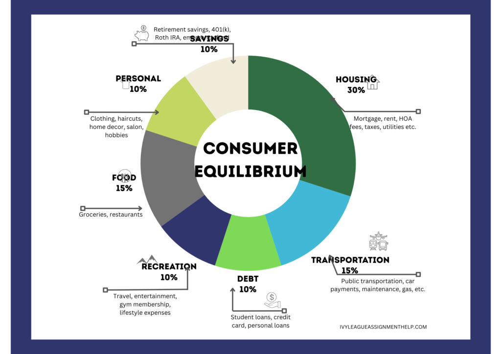
No Comments on Consumer Equilibrium: Balancing Preferences and Budget Constraints

Consumer equilibrium is a fundamental concept in microeconomics that explains how individuals make optimal purchasing decisions given their preferences and budget constraints. Understanding this concept is crucial for students and professionals alike, as it provides insights into consumer behavior, market dynamics, and personal finance management.

Key Takeaways

Consumer equilibrium occurs when a consumer maximizes utility within their budget constraint
It’s achieved when the marginal rate of substitution equals the price ratio of goods
Indifference curves and budget lines are key tools for visualizing consumer equilibrium
Changes in income or prices can shift the equilibrium point
Understanding consumer equilibrium helps in analyzing market demand and consumer choices

What is Consumer Equilibrium?

Consumer equilibrium is the state where a consumer has allocated their income in such a way that they cannot increase their total satisfaction or utility by changing their spending pattern. In other words, it’s the optimal combination of goods and services that a consumer can purchase given their preferences and budget constraints. At ivyleagueassignmenthelp.com we help and guide students to understand how this concept is central to understanding how consumers make choices in the marketplace and forms the foundation for analyzing demand curves and market behavior. For professionals in economics, business, and related fields, grasping consumer equilibrium is essential for developing insights into consumer behavior and market dynamics.

The Components of Consumer Equilibrium

To fully understand consumer equilibrium, we need to break it down into its key components:

Utility: The satisfaction or benefit a consumer derives from consuming a good or service.
Budget Constraint: The limit on consumer choices based on their income and the prices of goods.
Indifference Curves: Graphical representations of different combinations of goods that provide equal utility to a consumer.
Marginal Rate of Substitution (MRS): The rate at which a consumer is willing to give up one good for another while maintaining the same level of utility.

These components work together to determine the point of consumer equilibrium. For a more detailed explanation of these concepts, https://ivyleagueassignmenthelp.com/economic-assignment-help-economic-homework-help/

Conditions for Consumer Equilibrium

Achieving consumer equilibrium requires meeting specific conditions. These conditions ensure that the consumer is maximizing their utility given their budget constraint.

The Equimarginal Principle

The primary condition for consumer equilibrium is known as the equimarginal principle. This principle states that a consumer reaches equilibrium when the marginal utility per dollar spent is equal for all goods consumed.

Mathematically, this can be expressed as:

(MU₁ / P₁) = (MU₂ / P₂) = … = (MUₙ / Pₙ)

Where:

MU = Marginal Utility
P = Price
1, 2, …, n represent different goods

Good	Marginal Utility (MU)	Price	MU/P Ratio
X	10	$5	2
Y	8	$4	2
Z	6	$3	2

The Equimarginal Principle

This table indicates that each good has the same MU/P ratio, meaning the consumer derives the same utility per dollar spent on each good. This situation typically suggests that the consumer is in equilibrium, as the MU/P ratio is equal across all goods. In consumer equilibrium, the marginal utility per dollar spent should be the same for all goods to maximize total utility within a given budget. In this example, the consumer is in equilibrium because the MU/P ratio is equal for all goods.

Graphical Representation

Graphically, consumer equilibrium is represented by the point where an indifference curve is tangent to the budget line. This point of tangency ensures that:

The consumer is on the highest possible indifference curve given their budget constraint.
The slope of the indifference curve (MRS) equals the slope of the budget line (price ratio).

Factors Affecting Consumer Equilibrium

Several factors can influence consumer equilibrium, causing shifts in the optimal consumption bundle:

Changes in Income: An increase or decrease in income shifts the budget line, potentially leading to a new equilibrium point.
Price Changes: Alterations in the prices of goods can rotate the budget line, affecting the equilibrium.
Changes in Preferences: Shifts in consumer tastes can alter the shape of indifference curves, leading to a new equilibrium.
Introduction of New Products: New goods entering the market can reshape consumer preferences and budget allocation.

Understanding these factors is crucial for analyzing how market changes affect consumer behavior and overall demand.

Income and Substitution Effects

When prices change, two effects come into play that influence consumer equilibrium:

Income Effect: The change in consumption due to the change in purchasing power.
Substitution Effect: The change in consumption due to the change in relative prices.

Income and Substitution Effects

Effect	Price Increase	Price Decrease
Income Effect	Negative (can afford less)	Positive (can afford more)
Substitution Effect	Negative (substitute away)	Positive (substitute towards)

Income and Substitution Effects

Explanation:

Income Effect:

Price Increase: When the price of a good increases, the purchasing power of the consumer decreases, meaning they can afford less of the good, resulting in a negative income effect.
Price Decrease: When the price of a good decreases, the purchasing power of the consumer increases, meaning they can afford more of the good, resulting in a positive income effect.

Substitution Effect:

Price Increase: When the price of a good increases, consumers will substitute away from the more expensive good to a relatively cheaper alternative, resulting in a negative substitution effect.
Price Decrease: When the price of a good decreases, consumers will substitute towards the now cheaper good from a relatively more expensive alternative, resulting in a positive substitution effect.

These effects help explain why demand curves are typically downward-sloping and how consumers adjust their purchasing behavior in response to price changes. For a more in-depth analysis of income and substitution effects, check out this article from ivyleagueassignmenthelp.com

Understanding consumer equilibrium and its related concepts is essential for anyone studying economics or working in fields related to consumer behavior and market analysis. By grasping these principles, students and professionals can gain valuable insights into how individuals make purchasing decisions and how markets function as a whole.

Applications of Consumer Equilibrium Theory

Consumer equilibrium theory has wide-ranging applications in various fields, from business strategy to public policy. Let’s explore some of these practical applications:

Market Demand Analysis

Understanding consumer equilibrium helps businesses and economists predict market demand. By analyzing how changes in prices or income affect individual consumer equilibria, we can estimate overall market demand curves.

Price Change	Individual Effect	Market Effect
10% Increase	Shift to lower indifference curve	Decrease in quantity demanded
10% Decrease	Shift to higher indifference curve	Increase in quantity demanded

Market Demand Analysis

Explanation:

Price Change – 10% Increase:

Individual Effect: When the price of a good increases by 10%, the consumer will experience a shift to a lower indifference curve. This means that the consumer can achieve a lower level of overall satisfaction or utility because the increased price reduces their purchasing power.
Market Effect: On the market level, a 10% increase in price typically leads to a decrease in the quantity demanded. This is due to both the income effect (consumers can afford less) and the substitution effect (consumers substitute away from the more expensive good).

Price Change – 10% Decrease:

Individual Effect: When the price of a good decreases by 10%, the consumer will experience a shift to a higher indifference curve. This means that the consumer can achieve a higher level of overall satisfaction or utility because the decreased price increases their purchasing power.
Market Effect: On the market level, a 10% decrease in price typically leads to an increase in the quantity demanded. This is due to both the income effect (consumers can afford more) and the substitution effect (consumers substitute towards the cheaper good).

Product Pricing Strategies

Businesses use consumer equilibrium concepts to develop effective pricing strategies. By understanding how price changes affect consumer choices, companies can optimize their pricing to maximize revenue or market share. For instance, luxury brands often maintain high prices to cater to consumers whose equilibrium point lies on higher indifference curves, signaling prestige and exclusivity.

Public Policy and Welfare Analysis

Policymakers use consumer equilibrium theory to assess the impact of various policies on consumer welfare. For example, when analyzing the effects of taxes or subsidies, economists consider how these measures shift consumer equilibrium points.

Policy	Effect on Consumer Equilibrium	Welfare Impact
Sales Tax	Shifts budget line inward	Potentially negative
Subsidy	Shifts budget line outward	Potentially positive

Public Policy and Welfare Analysis

Explanation:

Sales Tax:

Effect on Consumer Equilibrium: A sales tax increases the prices of goods for the consumer, effectively reducing their real income. This causes the budget line to shift inward, meaning the consumer can afford less than before.
Welfare Impact: The welfare impact is potentially negative because consumers have less purchasing power, leading to lower utility or satisfaction levels.

Subsidy:

Effect on Consumer Equilibrium: A subsidy decreases the prices of goods for the consumer, effectively increasing their real income. This causes the budget line to shift outward, meaning the consumer can afford more than before.
Welfare Impact: The welfare impact is potentially positive because consumers have more purchasing power, leading to higher utility or satisfaction levels.

Advanced Concepts in Consumer Equilibrium

As we delve deeper into consumer equilibrium theory, several advanced concepts emerge that provide further insights into consumer behavior and market dynamics.

Revealed Preference Theory

Revealed preference theory, developed by economist Paul Samuelson, provides an alternative approach to analyzing consumer behavior. Instead of relying on unobservable utility functions, it infers preferences from observed choices. This theory argues that if a consumer chooses one bundle over another when both are affordable, the chosen bundle is revealed to be preferred. This approach has practical applications in empirical studies of consumer behavior.

Corner Solutions

In some cases, consumer equilibrium may occur at a “corner” of the budget line, rather than at a point of tangency with an indifference curve. This happens when a consumer spends their entire budget on one good, completely forgoing the other.

Consumption Scenarios and Equilibrium Types

Scenario	Equilibrium Type	Consumption Pattern
Normal	Tangency Solution	Mix of goods
Corner Solution	At budget line endpoint	All of one good, none of the other

Consumption Scenarios and Equilibrium Types

Explanation:

Normal Scenario:

Equilibrium Type: Tangency Solution
Consumption Pattern: In this scenario, the consumer chooses a mix of goods such that the indifference curve is tangent to the budget line. This represents a typical consumption pattern where the consumer spreads their spending across multiple goods to maximize utility.

Corner Solution:

Equilibrium Type: At budget line endpoint
Consumption Pattern: In this scenario, the consumer spends all their budget on one good and none on the other. This occurs when the marginal utility per dollar spent on one good is always higher than that of the other, leading the consumer to allocate all resources to the more preferred good.

Corner solutions are particularly relevant when analyzing consumer choices involving complementary goods or when dealing with extreme price differentials.

Consumer Equilibrium in Labor-Leisure Choices

The concept of consumer equilibrium can be extended to analyze how individuals allocate their time between work and leisure. In this model, individuals choose between earning income (which can be used to purchase goods) and enjoying leisure time. The equilibrium point represents the optimal work-leisure balance for an individual, given their preferences and the prevailing wage rate. This application of consumer equilibrium theory has important implications for labor economics and policy discussions around work hours and minimum wage laws.

Limitations and Criticisms of Consumer Equilibrium Theory

While consumer equilibrium theory provides valuable insights, it’s important to recognize its limitations:

Assumption of Rationality: The theory assumes consumers always make rational, consistent choices, which may not reflect real-world behavior.
Simplification: Most models consider only two goods, while real-world decisions often involve multiple goods and services.
Static Analysis: The theory provides a snapshot in time and doesn’t account for dynamic changes in preferences or circumstances.
Ignores Psychological Factors: Emotional and social influences on consumer choices are not directly incorporated into the model.

These limitations have led to the development of behavioral economics, which incorporates psychological insights into economic models to better explain and predict consumer behavior.

FAQs

Q: How does consumer equilibrium relate to the law of diminishing marginal utility? A: Consumer equilibrium is achieved when the marginal utility per dollar spent is equal across all goods, which is a direct application of the law of diminishing marginal utility.
Q: Can a consumer be in equilibrium if they don’t spend all their income? A: Yes, if saving provides more utility than spending on available goods, a consumer can be in equilibrium without spending all their income.
Q: How do behavioral economists view consumer equilibrium? A: Behavioral economists recognize the importance of consumer equilibrium but also consider psychological factors and cognitive biases that might cause deviations from traditional economic models.
Q: How does consumer equilibrium change in a multi-person household? A: In a multi-person household, the equilibrium becomes more complex as it needs to account for the preferences and utility of multiple individuals, often leading to negotiated or compromised consumption decisions.
Q: Can consumer equilibrium help explain brand loyalty? A: While traditional consumer equilibrium theory doesn’t directly address brand loyalty, extensions of the theory that incorporate factors like habit formation and psychological attachment can help explain why consumers might consistently choose one brand over others, even when prices change.

Understanding consumer equilibrium is crucial for anyone studying economics or working in fields related to consumer behavior and market analysis. By grasping these principles and their applications, students and professionals can gain valuable insights into how individuals make purchasing decisions, how markets function, and how various economic policies might impact consumer welfare.

QUICK QUOTE

Academic Level

Type of Paper

Number of Pages

Approximately 250 words

Urgency

$12

ORDER NOW

Benefits of Peer Study Groups and How They Enhance Learning
What Are Peer Study Groups? What is a Peer Study Group?A peer study group represents a dynamic learning approach where individuals,… Read more: Benefits of Peer Study Groups and How They Enhance Learning
Why Nursing Writing Help is Essential
Nursing students often face significant challenges when completing their academic assignments. Hiring a professional nursing writer can provide valuable assistance and… Read more: Why Nursing Writing Help is Essential
How to Organize Your Study Space for Maximum Productivity?
Effective study space organization is crucial for enhancing productivity and achieving academic success. Whether you’re a college student or a professional… Read more: How to Organize Your Study Space for Maximum Productivity?
What Are the Best Strategies for Tackling Last-Minute Assignments?
Procrastination is a common challenge for students and professionals alike. When faced with looming deadlines and mounting pressure, it’s crucial to… Read more: What Are the Best Strategies for Tackling Last-Minute Assignments?
The Ultimate Guide to Executive Summaries: Crafting Impactful Business Communications
An executive summary is a crucial component of business documents, providing a concise overview of a larger report or proposal. This… Read more: The Ultimate Guide to Executive Summaries: Crafting Impactful Business Communications

Tags Budget Constraints, Consumer Behavior, Economic Theory, Market Equilibrium, Preference Balancing

Economics

Engel’s Law: Understanding the Concept and Its Applications

Post author By Evans
Post date July 11, 2024
No Comments on Engel’s Law: Understanding the Concept and Its Applications

Key Takeaways

Understanding Engel’s Law
Applications in economics and consumer behavior
Historical context and development

Introduction to Engel’s Law

Engel’s Law is a fundamental concept in economics that describes how household expenditure on a particular good or service varies with changes in income. At ivyleagueassignmenthelp.com we help and guide students to understand how this law provides insights into consumer behavior and helps in understanding economic trends and policy making.

Definition of Engel’s Law

What is Engel’s Law?

Engel’s Law states that as household income increases, the proportion of income spent on food decreases, even if the actual expenditure on food rises. This implies that food consumption is a necessity, and as people become wealthier, they spend a smaller percentage of their total income on food and more on non-essential items.

Historical Context of Engel’s Law

Ernst Engel, a German statistician, formulated this law in the 19th century. He observed and analyzed household expenditure patterns and concluded that income elasticity varies across different categories of goods. Engel’s work laid the foundation for further studies in consumer behavior and economic planning.

Engel’s Law in Historical Context

Year	Economist	Contribution
1857	Ernst Engel	Formulated Engel’s Law
1930	John Maynard Keynes	Expanded on household spending patterns

Components of Engel’s Law

Income and Spending Patterns

Engel’s Law highlights the relationship between income levels and spending patterns. As income increases, households allocate a smaller proportion of their budget to necessities like food and a larger proportion to luxuries and discretionary items.

Changes in Expenditure as Income Rises

With rising income, absolute spending on food may increase, but the percentage of total income spent on food decreases. Conversely, spending on luxury items increases both in absolute terms and as a percentage of income.

Distinction Between Necessities and Luxuries

Engel’s Law helps distinguish between necessities (e.g., food, basic clothing) and luxuries (e.g., entertainment, travel). Necessities have a lower income elasticity of demand compared to luxuries, which have a higher income elasticity.

Spending Patterns by Income Level

Income Level	Food (% of Income)	Luxuries (% of Income)
Low	60%	10%
Medium	40%	20%
High	20%	40%

Graphical Representation of Engel’s Law

Engel Curves

Engel curves graphically represent the relationship between income and expenditure on a particular good. These curves show how spending on different categories of goods changes as income rises.

Engel Curve for Food

Income	Food Expenditure
$1000	$600
$2000	$800
$3000	$900

Engel Curve for Food

Applications of Engel’s Law in Economics

Consumer Spending Analysis

Engel’s Law is crucial for analyzing consumer spending patterns. It helps economists and policymakers understand how changes in income affect household expenditure and consumption trends.

Policy Making and Economic Planning

Governments and organizations use insights from Engel’s Law to design economic policies, such as tax structures, social welfare programs, and subsidies. Understanding spending patterns helps in targeting interventions effectively.

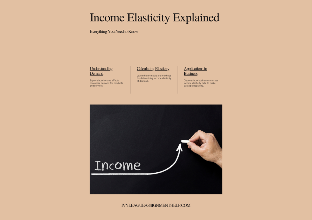
Income Elasticity of Demand

Engel’s Law provides a basis for calculating income elasticity of demand, which measures how the quantity demanded of a good responds to changes in income. This is vital for market analysis and business strategy.

Income Elasticity Calculation

Income Change	Food Demand Change	Elasticity
+10%	+5%	0.5
+20%	+8%	0.4

Income Elasticity Calculation

Factors Influencing Engel’s Law

Income Levels

The primary factor influencing Engel’s Law is the level of household income. As income rises, spending patterns shift from necessities to luxuries.

Cultural Differences

Cultural factors can affect spending patterns. For example, in cultures where food plays a central role, the proportion of income spent on food may remain higher even as income rises.

Changes in Prices

Inflation and changes in the prices of goods can influence the applicability of Engel’s Law. Rising food prices might mean a higher proportion of income is spent on food, even with increasing income.

Real-World Examples of Engel’s Law

Case Studies

Developing vs. Developed Countries

In developing countries, a larger proportion of income is spent on food compared to developed countries. As economies grow and incomes rise, the expenditure patterns shift towards more discretionary spending.

Impact on Food Expenditure

In high-income households, spending on food might increase in absolute terms, but it decreases as a proportion of total income. This reflects the shift towards higher spending on luxury goods and services.

Engel’s Law in Different Economies

Country	Income Level	Food (% of Income)	Luxuries (% of Income)
Developing	Low	50%	10%
Developed	High	20%	30%

Engel’s Law in Different Economies

Frequently Asked Questions

How does Engel’s Law affect consumer behavior?

Engel’s Law affects consumer behavior by influencing how households allocate their budget. With rising incomes, people spend a smaller percentage on food and more on other goods and services, enhancing their standard of living.

What are the components of Engel’s Law?

The components of Engel’s Law include income elasticity of demand, expenditure patterns, and the classification of goods into necessities, normal goods, and luxury items.

How is Engel’s Law represented graphically?

Engel’s Law is represented graphically through Engel Curves, which plot the relationship between income and expenditure on specific goods. These curves typically slope upwards for normal goods and flatten for necessities.

What factors influence Engel’s Law?

Factors influencing Engel’s Law include income levels, cultural factors, price changes, and technological advancements, all of which can affect household spending patterns.

What are some real-world examples of Engel’s Law?

Real-world examples of Engel’s Law can be seen in the spending patterns of developed and developing countries. In developed nations, a smaller proportion of income is spent on food, while in developing countries, food expenditure constitutes a larger share of household budgets.

QUICK QUOTE

Academic Level

Type of Paper

Number of Pages

Approximately 250 words

Urgency

$12

ORDER NOW

Benefits of Peer Study Groups and How They Enhance Learning
What Are Peer Study Groups? What is a Peer Study Group?A peer study group represents a dynamic learning approach where individuals,… Read more: Benefits of Peer Study Groups and How They Enhance Learning
Why Nursing Writing Help is Essential
Nursing students often face significant challenges when completing their academic assignments. Hiring a professional nursing writer can provide valuable assistance and… Read more: Why Nursing Writing Help is Essential
How to Organize Your Study Space for Maximum Productivity?
Effective study space organization is crucial for enhancing productivity and achieving academic success. Whether you’re a college student or a professional… Read more: How to Organize Your Study Space for Maximum Productivity?
What Are the Best Strategies for Tackling Last-Minute Assignments?
Procrastination is a common challenge for students and professionals alike. When faced with looming deadlines and mounting pressure, it’s crucial to… Read more: What Are the Best Strategies for Tackling Last-Minute Assignments?
The Ultimate Guide to Executive Summaries: Crafting Impactful Business Communications
An executive summary is a crucial component of business documents, providing a concise overview of a larger report or proposal. This… Read more: The Ultimate Guide to Executive Summaries: Crafting Impactful Business Communications

Tags Consumer Behavior, Economic Theory, Engel's Law, Expenditure Patterns, Income Elasticity

Economics

Price Elasticity of Demand: Comprehensive Analysis

Post author By Evans
Post date July 11, 2024
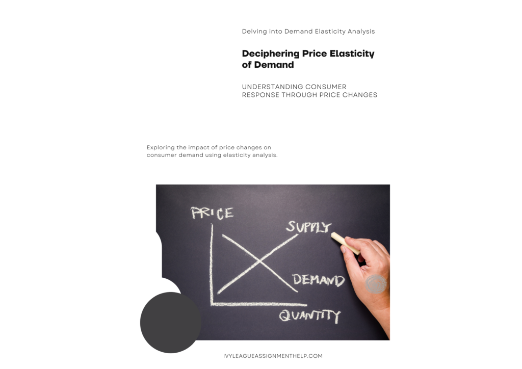
No Comments on Price Elasticity of Demand: Comprehensive Analysis

Key Takeaways:

Price elasticity of demand measures how quantity demanded changes with price fluctuations.
Various factors, such as the availability of substitutes and the proportion of income spent on the good, influence price elasticity.
Understanding price elasticity helps businesses set optimal prices and predict consumer behavior.

Introduction

Understanding price elasticity of demand is essential for businesses, economists, and policymakers. It provides insights into how sensitive consumers are to price changes, which can guide pricing strategies, revenue management, and economic policies. At ivyleagueassignmenthelp.com we help and guide students to explore the various aspects of price elasticity of demand, including its determinants, types, and applications in different markets.

Definition of Price Elasticity of Demand

Price elasticity of demand (PED) is a measure that indicates the responsiveness of the quantity demanded of a good to a change in its price. It is calculated as the percentage change in quantity demanded divided by the percentage change in price. A higher elasticity value indicates greater sensitivity to price changes.

Importance of Price Elasticity of Demand

Understanding PED is crucial for several reasons:

It helps businesses set prices that maximize revenue and profits.
It allows policymakers to predict the effects of taxation and regulation on consumption.
It aids in understanding consumer behavior and market dynamics.

Determinants of Price Elasticity of Demand

Availability of Substitutes

The presence of close substitutes makes demand more elastic. When consumers can easily switch to another product if the price of one product rises, the demand for the initial product becomes more sensitive to price changes.

Proportion of Income Spent on the Good

Goods that take up a significant portion of a consumer’s income tend to have more elastic demand. Price changes for these goods significantly impact the consumer’s budget, leading to greater sensitivity.

Necessity vs. Luxury

Necessities usually have inelastic demand because consumers need them regardless of price changes, whereas luxuries have more elastic demand since consumers can forego these goods if prices rise.

Time Horizon

Demand elasticity can vary over time. In the short term, demand is usually inelastic because consumers need time to adjust their behavior. Over the long term, they can find substitutes or change consumption habits, making demand more elastic.

Calculating Price Elasticity of Demand

Formula for Price Elasticity of Demand

The formula for calculating price elasticity of demand is: Price Elasticity of Demand=% Change in Quantity Demanded% Change in Price\text{Price Elasticity of Demand} = \frac{\% \text{ Change in Quantity Demanded}}{\% \text{ Change in Price}}Price Elasticity of Demand=% Change in Price% Change in Quantity Demanded

Interpreting the Coefficient

If the coefficient is greater than 1, demand is elastic.
If the coefficient is less than 1, demand is inelastic.
If the coefficient is equal to 1, demand is unitary elastic.

Examples of Price Elasticity Calculation

For instance, if the price of a product increases by 10% and the quantity demanded decreases by 20%, the price elasticity of demand would be: −20%10%=−2\frac{-20\%}{10\%} = -210%−20%=−2 This indicates elastic demand.

Types of Price Elasticity of Demand

Elastic Demand

Elastic demand occurs when the price elasticity of demand is greater than 1. Small changes in price lead to significant changes in quantity demanded.

Inelastic Demand

Inelastic demand happens when the price elasticity is less than 1. Price changes have little impact on the quantity demanded.

Unitary Elastic Demand

When the price elasticity is exactly 1, it is termed unitary elastic. The percentage change in quantity demanded is equal to the percentage change in price.

Perfectly Elastic Demand

In cases of perfectly elastic demand, any change in price results in an infinite change in quantity demanded. This is rare and typically theoretical.

Perfectly Inelastic Demand

Perfectly inelastic demand means that quantity demanded remains constant regardless of price changes. This is also rare and theoretical.

Factors Influencing Price Elasticity

Consumer Preferences

Changes in consumer preferences can make demand more or less elastic. For example, trends can temporarily increase the elasticity of demand for fashionable items.

Market Conditions

Market conditions, including competition and market structure, significantly influence price elasticity. More competitive markets tend to have more elastic demand.

Economic Environment

The broader economic environment, including factors like inflation and employment rates, also affects price elasticity. During economic downturns, demand tends to become more elastic.

Price Elasticity of Demand in Different Markets

Price Elasticity in Competitive Markets

In highly competitive markets, consumers have more choices, making demand more elastic. Companies must be cautious with pricing strategies to avoid losing market share.

Price Elasticity in Monopolistic Markets

Monopolistic markets, where one firm dominates, tend to have inelastic demand. Consumers have fewer alternatives, allowing the firm more pricing power.

Price Elasticity in Oligopolistic Markets

Oligopolistic markets, with a few dominant firms, exhibit varying elasticities. Firms often engage in strategic pricing, considering the potential responses of competitors.

Good/Service	Price Elasticity
Bread	Inelastic
Gasoline	Inelastic
Electronics	Elastic
Luxury Cars	Elastic

Price Elasticity of Common Goods and Services

Applications of Price Elasticity of Demand

Pricing Strategies

Businesses use price elasticity to set optimal prices. Understanding whether demand is elastic or inelastic helps in determining the potential impact of price changes.

Revenue Management

Price elasticity is crucial in revenue management. Companies analyze it to maximize revenue by adjusting prices based on demand sensitivity.

Taxation Policies

Governments consider price elasticity when designing taxation policies. Goods with inelastic demand, like gasoline, often have higher taxes because consumers are less sensitive to price changes.

Real-World Examples

Price Elasticity in the Tech Industry

In the tech industry, demand for products like smartphones is relatively elastic. Price changes can significantly affect sales, as consumers have many alternatives.

Price Elasticity in the Automotive Industry

The automotive industry exhibits varying elasticity. Luxury cars tend to have more elastic demand compared to essential models, where demand is relatively inelastic.

Price Elasticity in the Pharmaceutical Industry

Pharmaceuticals often have inelastic demand. Life-saving drugs, for instance, maintain constant demand regardless of price changes due to their necessity.

Applications of Price Elasticity of Demand

Pricing Strategies

Businesses use price elasticity to set optimal prices. Understanding whether demand is elastic or inelastic helps in determining the potential impact of price changes. For instance, inelastic demand allows firms to increase prices without significantly reducing sales, thereby increasing revenue.

Revenue Management

Price elasticity is crucial in revenue management. Companies analyze it to maximize revenue by adjusting prices based on demand sensitivity. For example, airlines use price elasticity to adjust ticket prices in response to demand fluctuations.

Taxation Policies

Governments consider price elasticity when designing taxation policies. Goods with inelastic demand, like gasoline, often have higher taxes because consumers are less sensitive to price changes. This ensures steady tax revenue despite price increases.

Real-World Examples

Price Elasticity in the Tech Industry

In the tech industry, demand for products like smartphones is relatively elastic. Price changes can significantly affect sales, as consumers have many alternatives. For example, a 10% price drop in a popular smartphone model can lead to a significant increase in sales volume.

Price Elasticity in the Automotive Industry

The automotive industry exhibits varying elasticity. Luxury cars tend to have more elastic demand compared to essential models, where demand is relatively inelastic. Price reductions in luxury vehicles can lead to a noticeable increase in sales, whereas essential car models have steady demand regardless of price changes.

Price Elasticity in the Pharmaceutical Industry

Pharmaceuticals often have inelastic demand. Life-saving drugs, for instance, maintain constant demand regardless of price changes due to their necessity. This inelastic nature means that price increases do not significantly reduce the quantity demanded

Frequently Asked Questions

What does a price elasticity of -1 mean?

A price elasticity of -1 indicates unitary elasticity. This means that a 1% increase in price leads to a 1% decrease in quantity demanded, and vice versa. Revenue remains unchanged as the price and quantity demanded move proportionally.

How is price elasticity used in business?

Businesses use price elasticity to determine pricing strategies. By understanding the elasticity of their products, companies can predict how changes in price will affect sales volume and revenue. This helps in setting optimal prices to maximize profits.

Can price elasticity be positive?

Price elasticity of demand is typically negative, reflecting the inverse relationship between price and quantity demanded. However, in rare cases, it can be positive for certain luxury or status goods, where higher prices may increase demand due to perceived exclusivity.

What factors make demand more elastic?

Several factors can make demand more elastic, including the availability of substitutes, a higher proportion of income spent on the good, and the good being a luxury rather than a necessity. Additionally, demand tends to be more elastic over longer time horizons as consumers find alternatives.

How does price elasticity relate to total revenue?

Price elasticity directly impacts total revenue. If demand is elastic, a price increase will decrease total revenue, while a price decrease will increase total revenue. Conversely, if demand is inelastic, a price increase will increase total revenue, and a price decrease will decrease total revenue.

QUICK QUOTE

Academic Level

Type of Paper

Number of Pages

Approximately 250 words

Urgency

$12

ORDER NOW

Benefits of Peer Study Groups and How They Enhance Learning
What Are Peer Study Groups? What is a Peer Study Group?A peer study group represents a dynamic learning approach where individuals,… Read more: Benefits of Peer Study Groups and How They Enhance Learning
Why Nursing Writing Help is Essential
Nursing students often face significant challenges when completing their academic assignments. Hiring a professional nursing writer can provide valuable assistance and… Read more: Why Nursing Writing Help is Essential
How to Organize Your Study Space for Maximum Productivity?
Effective study space organization is crucial for enhancing productivity and achieving academic success. Whether you’re a college student or a professional… Read more: How to Organize Your Study Space for Maximum Productivity?
What Are the Best Strategies for Tackling Last-Minute Assignments?
Procrastination is a common challenge for students and professionals alike. When faced with looming deadlines and mounting pressure, it’s crucial to… Read more: What Are the Best Strategies for Tackling Last-Minute Assignments?
The Ultimate Guide to Executive Summaries: Crafting Impactful Business Communications
An executive summary is a crucial component of business documents, providing a concise overview of a larger report or proposal. This… Read more: The Ultimate Guide to Executive Summaries: Crafting Impactful Business Communications

Tags Demand Analysis, Economic Elasticity, Market Dynamics, Price Elasticity of Demand, Pricing Strategies

Economics

Income Elasticity of Demand: A Comprehensive Guide

Post author By Evans
Post date July 11, 2024
No Comments on Income Elasticity of Demand: A Comprehensive Guide

Key Takeaways:

Income elasticity of demand measures how the quantity demanded of a good responds to changes in consumer income.
Various factors, such as the type of good and consumer preferences, influence income elasticity.
Understanding income elasticity helps businesses and policymakers predict changes in demand based on economic conditions.

Introduction

Understanding income elasticity of demand is vital for businesses, economists, and policymakers. It provides insights into how changes in consumer income affect the quantity demanded of goods and services. By analyzing income elasticity, companies can make informed decisions about product offerings, pricing strategies, and market segmentation. At ivyleagueassignmenthelp.com we help and guide students to delve into the various aspects of income elasticity of demand, including its determinants, types, and real-world.

Definition of Income Elasticity of Demand

Income elasticity of demand (YED) measures the responsiveness of the quantity demanded of a good to a change in consumer income. It is calculated as the percentage change in quantity demanded divided by the percentage change in income. A higher elasticity value indicates greater sensitivity to income changes.

Importance of Income Elasticity of Demand

Understanding YED is crucial for several reasons:

It helps businesses forecast demand based on economic trends.
It allows policymakers to predict the effects of economic policies on consumption.
It aids in identifying which goods are necessities and which are luxuries.

Determinants of Income Elasticity of Demand

Type of Good

Goods can be classified based on their income elasticity:

Normal Goods: These goods have a positive income elasticity, meaning that as income increases, the quantity demanded also increases. Examples include electronics and dining out.
Inferior Goods: These goods have a negative income elasticity, meaning that as income increases, the quantity demanded decreases. Examples include generic brands and public transportation.

Consumer Preferences

Changes in consumer preferences can significantly affect income elasticity. For example, a shift towards healthier lifestyles can increase the income elasticity of organic food products.

Income Level

The income level of consumers also influences elasticity. Higher-income consumers may exhibit different demand patterns compared to lower-income consumers. For instance, luxury goods may have high income elasticity among wealthy consumers but low or negative elasticity among lower-income groups.

Calculating Income Elasticity of Demand

Formula for Income Elasticity of Demand

The formula for calculating income elasticity of demand is: Income Elasticity of Demand=% Change in Quantity Demanded% Change in Income\text{Income Elasticity of Demand} = \frac{\% \text{ Change in Quantity Demanded}}{\% \text{ Change in Income}}Income Elasticity of Demand=% Change in Income% Change in Quantity Demanded

Interpreting the Coefficient

Positive YED (>1): Luxury goods, which are highly sensitive to income changes.
Positive YED (<1): Necessities, which are less sensitive to income changes.
Negative YED: Inferior goods, where demand decreases as income rises.

Examples of Income Elasticity Calculation

For example, if consumer income increases by 10% and the quantity demanded for luxury cars increases by 25%, the income elasticity of demand would be: 25%10%=2.5\frac{25\%}{10\%} = 2.510%25%=2.5 This indicates that luxury cars are highly income elastic.

Types of Income Elasticity of Demand

High Income Elasticity of Demand

Goods with high income elasticity (greater than 1) are typically luxury items. Their demand increases more than proportionally as income rises.

Low Income Elasticity of Demand

Goods with low income elasticity (less than 1 but greater than 0) are necessities. Their demand increases with income, but at a slower rate.

Negative Income Elasticity of Demand

Goods with negative income elasticity are inferior goods. As income increases, the demand for these goods decreases.

Factors Influencing Income Elasticity

Market Trends

Market trends and economic conditions can influence income elasticity. For example, during economic booms, the demand for luxury goods may increase significantly.

Cultural Factors

Cultural factors and social norms can also impact income elasticity. In some cultures, certain goods may be viewed as status symbols, increasing their income elasticity.

Technological Advancements

Technological advancements can change the income elasticity of certain goods. For example, new technologies can make luxury items more accessible, altering their demand patterns.

Income Elasticity of Demand in Different Markets

Income Elasticity in Developed Markets

In developed markets, consumers typically have higher disposable incomes, leading to greater demand for luxury goods. The income elasticity for such goods is often higher.

Income Elasticity in Developing Markets

In developing markets, the focus is more on necessities and basic goods. The income elasticity for these goods tends to be lower, reflecting the prioritization of essential items over luxury products.

Year	Product	Elasticity Coefficient
2020	Organic Foods	1.2
2021	Luxury Goods	2.0
2022	Generic Brands	-0.5

Historical Income Elasticity Data

Applications of Income Elasticity of Demand

Product Development

Understanding income elasticity helps businesses develop products that meet the changing demands of consumers. For instance, during economic growth, companies might introduce more premium products.

Market Segmentation

Businesses use income elasticity to segment markets effectively. By identifying which goods are viewed as necessities or luxuries, companies can tailor their marketing strategies to different income groups.

Policy Making

Policymakers use income elasticity to predict the impact of economic policies on consumption. For example, tax cuts for middle-income families might lead to increased demand for certain goods.

Real-World Examples

Income Elasticity in the Automotive Industry

In the automotive industry, luxury cars exhibit high income elasticity. As consumer incomes rise, the demand for premium and luxury vehicles increases significantly.

Income Elasticity in the Food Industry

The food industry shows varying income elasticity. Basic staples like rice and bread have low income elasticity, while organic and gourmet foods have higher income elasticity.

Income Elasticity in the Technology Sector

In the technology sector, products like high-end smartphones and laptops have high income elasticity. Consumers are more likely to purchase the latest models as their incomes increase.

Income Elasticity of Common Goods and Services

Good/Service	Income Elasticity
Basic Groceries	Low
Luxury Cars	High
Public Transportation	Negative
High-End Electronics	High

Income Elasticity of Common Goods and Services

Historical Income Elasticity Data

Frequently Asked Questions

What is income elasticity of demand?

Income elasticity of demand measures how the quantity demanded of a good responds to changes in consumer income. It indicates whether a good is a necessity, luxury, or inferior.

How is income elasticity of demand calculated?

Income elasticity of demand is calculated using the formula: Income Elasticity of Demand=% Change in Quantity Demanded% Change in Income\text{Income Elasticity of Demand} = \frac{\% \text{ Change in Quantity Demanded}}{\% \text{ Change in Income}}Income Elasticity of Demand=% Change in Income% Change in Quantity Demanded

Why is understanding income elasticity important for businesses?

Understanding income elasticity helps businesses forecast demand, develop products, and set pricing strategies. It also aids in market segmentation and targeting different income groups.

What are some examples of goods with high income elasticity?

Examples of goods with high income elasticity include luxury cars, high-end electronics, and premium foods. These goods see a significant increase in demand as consumer incomes rise.

How does income elasticity differ in developed and developing markets?

In developed markets, consumers have higher disposable incomes, leading to greater demand for luxury goods. In developing markets, the focus is more on necessities, resulting in lower income elasticity for basic goods.

QUICK QUOTE

Academic Level

Type of Paper

Number of Pages

Approximately 250 words

Urgency

$12

ORDER NOW

Benefits of Peer Study Groups and How They Enhance Learning
What Are Peer Study Groups? What is a Peer Study Group?A peer study group represents a dynamic learning approach where individuals,… Read more: Benefits of Peer Study Groups and How They Enhance Learning
Why Nursing Writing Help is Essential
Nursing students often face significant challenges when completing their academic assignments. Hiring a professional nursing writer can provide valuable assistance and… Read more: Why Nursing Writing Help is Essential
How to Organize Your Study Space for Maximum Productivity?
Effective study space organization is crucial for enhancing productivity and achieving academic success. Whether you’re a college student or a professional… Read more: How to Organize Your Study Space for Maximum Productivity?
What Are the Best Strategies for Tackling Last-Minute Assignments?
Procrastination is a common challenge for students and professionals alike. When faced with looming deadlines and mounting pressure, it’s crucial to… Read more: What Are the Best Strategies for Tackling Last-Minute Assignments?
The Ultimate Guide to Executive Summaries: Crafting Impactful Business Communications
An executive summary is a crucial component of business documents, providing a concise overview of a larger report or proposal. This… Read more: The Ultimate Guide to Executive Summaries: Crafting Impactful Business Communications

Tags Consumer Demand, Economic Analysis, Income Elasticity, Luxury and Necessity Goods, Market Segmentation

Economics

Understanding Cross-Price Elasticity of Demand

Post author By Evans
Post date July 11, 2024
No Comments on Understanding Cross-Price Elasticity of Demand

Key Takeaways:

Cross-price elasticity of demand measures how the quantity demanded of one good responds to a change in the price of another good.
Different types of goods, such as substitutes and complements, have varying cross-price elasticity.
Understanding cross-price elasticity helps businesses and policymakers make informed decisions about pricing and market strategies.

Definition of Cross-Price Elasticity of Demand

Cross-price elasticity of demand (XED) measures the responsiveness of the quantity demanded of one good to a change in the price of another good. It is calculated as the percentage change in the quantity demanded of the first good divided by the percentage change in the price of the second good.

Importance of Cross-Price Elasticity of Demand

Understanding XED is essential for several reasons:

It helps businesses understand the relationship between their products and those of competitors or complementary goods.
It allows policymakers to predict the effects of price changes on market demand and overall economic welfare.
It aids in strategic decision-making for pricing, marketing, and inventory management.

Determinants of Cross-Price Elasticity of Demand

Substitute Goods

Substitute goods are products that can replace each other. A positive cross-price elasticity indicates that an increase in the price of one good leads to an increase in the quantity demanded of its substitute.

Complementary Goods

Complementary goods are products that are consumed together. A negative cross-price elasticity means that an increase in the price of one good leads to a decrease in the quantity demanded of its complement.

Independent Goods

Independent goods have no significant relationship, so a change in the price of one good does not affect the demand for the other. The cross-price elasticity for these goods is zero or close to zero.

Calculating Cross-Price Elasticity of Demand

Formula for Cross-Price Elasticity of Demand

The formula for calculating cross-price elasticity of demand is: Cross-Price Elasticity of Demand=% Change in Quantity Demanded of Good A% Change in Price of Good B\text{Cross-Price Elasticity of Demand} = \frac{\% \text{ Change in Quantity Demanded of Good A}}{\% \text{ Change in Price of Good B}}Cross-Price Elasticity of Demand=% Change in Price of Good B% Change in Quantity Demanded of Good A

Interpreting the Coefficient

Positive XED: Indicates that the goods are substitutes.
Negative XED: Indicates that the goods are complements.
Zero XED: Indicates that the goods are independent.

Examples of Cross-Price Elasticity Calculation

For instance, if the price of tea increases by 10% and the quantity demanded for coffee increases by 5%, the cross-price elasticity of demand would be: 5%10%=0.5\frac{5\%}{10\%} = 0.510%5%=0.5 This indicates that tea and coffee are substitutes.

Types of Cross-Price Elasticity of Demand

Positive Cross-Price Elasticity

Positive cross-price elasticity occurs when the demand for one good increases as the price of another good rises, indicating a substitute relationship.

Negative Cross-Price Elasticity

Negative cross-price elasticity occurs when the demand for one good decreases as the price of another good rises, indicating a complementary relationship.

Zero Cross-Price Elasticity

Zero cross-price elasticity occurs when the demand for one good is unaffected by changes in the price of another good, indicating an independent relationship.

Factors Influencing Cross-Price Elasticity

Consumer Preferences

Changes in consumer preferences can significantly affect cross-price elasticity. For example, if consumers develop a preference for healthier options, the cross-price elasticity between sugary drinks and health drinks may change.

Market Conditions

Market conditions, including competition and market structure, play a significant role in cross-price elasticity. In highly competitive markets, the elasticity between substitute goods may be higher.

Economic Environment

The broader economic environment, including factors like inflation and employment rates, also affects cross-price elasticity. During economic downturns, the elasticity between goods may become more pronounced as consumers look for cheaper alternatives.

Cross-Price Elasticity of Demand in Different Markets

Competitive Markets

In competitive markets, cross-price elasticity is often higher because consumers have more alternatives. Companies need to be aware of how their pricing strategies impact the demand for substitute products.

Monopolistic Markets

Oligopolistic Markets

Oligopolistic markets, with a few dominant firms, exhibit varying cross-price elasticities. Firms often engage in strategic pricing, considering the potential responses of competitors.

Applications of Cross-Price Elasticity of Demand

Pricing Strategies

Businesses use cross-price elasticity to set optimal prices for their products. Understanding the relationships between products helps in determining how price changes will impact demand and revenue.

Revenue Management

Cross-price elasticity is crucial in revenue management. Companies analyze it to maximize revenue by adjusting prices based on the relationships between their products and those of competitors.

Marketing Strategies

Real-World Examples

Cross-Price Elasticity in the Tech Industry

Cross-Price Elasticity in the Food Industry

The food industry shows varying cross-price elasticity. For example, a price increase in coffee may lead to higher demand for tea, indicating that these goods are substitutes.

Cross-Price Elasticity in the Automotive Industry

In the automotive industry, the cross-price elasticity between gasoline and electric cars is crucial. An increase in gasoline prices can boost the demand for electric vehicles.

Cross-Price Elasticity of Common Goods and Services

Good/Service	Cross-Price Elasticity
Tea and Coffee	Positive
Smartphones and Apps	Positive
Gasoline and Electric Cars	Negative
Bread and Butter	Negative

Cross-Price Elasticity of Common Goods and Services

Historical Cross-Price Elasticity Data

Year	Product Pair	Elasticity Coefficient
2020	Coffee and Tea	0.6
2021	Gasoline and Electric Cars	-1.2
2022	Smartphones and Accessories	1.1

Historical Cross-Price Elasticity Data

Factors Influencing Cross-Price Elasticity

Consumer Preferences

Market Conditions

Market conditions, including competition and market structure, play a significant role in cross-price elasticity. In highly competitive markets, the elasticity between substitute goods may be higher. Businesses need to monitor their competitors’ pricing strategies closely.

Economic Environment

Cross-Price Elasticity of Demand in Different Markets

Competitive Markets

In competitive markets, cross-price elasticity is often higher because consumers have more alternatives. Companies must be aware of how their pricing strategies impact the demand for substitute products. For example, in the retail industry, a price increase by one brand can lead to a significant shift in demand to competing brands.

Monopolistic Markets

In monopolistic markets, where one firm dominates, cross-price elasticity tends to be lower. Consumers have fewer alternatives, which can reduce the sensitivity to price changes of complementary goods. For instance, a monopolistic telecom company may not experience significant demand shifts for its services despite price changes.

Oligopolistic Markets

Oligopolistic markets, with a few dominant firms, exhibit varying cross-price elasticities. Firms often engage in strategic pricing, considering the potential responses of competitors. For example, in the airline industry, price changes by one airline can significantly impact the demand for other airlines’ tickets.

Applications of Cross-Price Elasticity of Demand

Pricing Strategies

Businesses use cross-price elasticity to set optimal prices for their products. Understanding the relationships between products helps in determining how price changes will impact demand and revenue. For instance, a tech company might lower the price of its flagship smartphone to increase the demand for its accessories.

Revenue Management

Cross-price elasticity is crucial in revenue management. Companies analyze it to maximize revenue by adjusting prices based on the relationships between their products and those of competitors. Retail chains, for example, use cross-price elasticity data to optimize pricing across product lines.

Marketing Strategies

Marketers use cross-price elasticity to develop effective marketing strategies. By understanding how changes in the price of one product affect the demand for another, they can create targeted promotions and pricing bundles. For example, grocery stores may bundle complementary products like bread and butter at a discounted price.

Real-World Examples

Cross-Price Elasticity in the Tech Industry

In the tech industry, products like smartphones and apps exhibit significant cross-price elasticity. A price drop in a popular smartphone model can increase the demand for compatible apps and accessories. This relationship helps tech companies develop pricing strategies that enhance overall sales.

Cross-Price Elasticity in the Food Industry

The food industry shows varying cross-price elasticity. For example, a price increase in coffee may lead to higher demand for tea, indicating that these goods are substitutes. On the other hand, a price increase in bread may reduce the demand for butter, highlighting their complementary nature.

Cross-Price Elasticity in the Automotive Industry

In the automotive industry, the cross-price elasticity between gasoline and electric cars is crucial. An increase in gasoline prices can boost the demand for electric vehicles. This relationship is essential for car manufacturers and policymakers focusing on sustainable transportation solutions.

Frequently Asked Questions

What does a cross-price elasticity of -1 mean?

A cross-price elasticity of -1 indicates that the goods are perfect complements. This means that a 1% increase in the price of one good leads to a 1% decrease in the quantity demanded of the complementary good. For example, if the price of printers increases by 1%, the demand for printer ink decreases by 1%.

How is cross-price elasticity used in economics?

Cross-price elasticity is used in economics to understand the relationships between different goods and how changes in the price of one good affect the demand for another. It helps in analyzing market competition, consumer behavior, and the impact of pricing strategies on overall demand.

What are the key determinants of cross-price elasticity?

The key determinants of cross-price elasticity include:

Type of Goods: Whether they are substitutes, complements, or independent goods.
Consumer Preferences: Changes in consumer tastes and preferences.
Market Conditions: The level of competition and market structure.
Economic Environment: Factors like inflation, employment rates, and overall economic health.

Can cross-price elasticity be positive?

Yes, cross-price elasticity can be positive when the goods in question are substitutes. This means that an increase in the price of one good leads to an increase in the quantity demanded of its substitute. For instance, if the price of butter rises, the demand for margarine may increase.

How does cross-price elasticity relate to consumer behavior?

Cross-price elasticity relates to consumer behavior by indicating how consumers substitute between different goods when prices change. It reflects the degree of substitutability or complementarity between products, helping businesses and policymakers understand and predict shifts in consumer demand.

QUICK QUOTE

Academic Level

Type of Paper

Number of Pages

Approximately 250 words

Urgency

$12

ORDER NOW

Benefits of Peer Study Groups and How They Enhance Learning
What Are Peer Study Groups? What is a Peer Study Group?A peer study group represents a dynamic learning approach where individuals,… Read more: Benefits of Peer Study Groups and How They Enhance Learning
Why Nursing Writing Help is Essential
Nursing students often face significant challenges when completing their academic assignments. Hiring a professional nursing writer can provide valuable assistance and… Read more: Why Nursing Writing Help is Essential
How to Organize Your Study Space for Maximum Productivity?
Effective study space organization is crucial for enhancing productivity and achieving academic success. Whether you’re a college student or a professional… Read more: How to Organize Your Study Space for Maximum Productivity?
What Are the Best Strategies for Tackling Last-Minute Assignments?
Procrastination is a common challenge for students and professionals alike. When faced with looming deadlines and mounting pressure, it’s crucial to… Read more: What Are the Best Strategies for Tackling Last-Minute Assignments?
The Ultimate Guide to Executive Summaries: Crafting Impactful Business Communications
An executive summary is a crucial component of business documents, providing a concise overview of a larger report or proposal. This… Read more: The Ultimate Guide to Executive Summaries: Crafting Impactful Business Communications

Tags Complementary Goods, Cross-Price Elasticity, Market Analysis, Pricing Strategies, Substitute Goods

Economics

Rational Consumer Behavior: Comprehensive Analysis

Post author By Evans
Post date July 11, 2024
No Comments on Rational Consumer Behavior: Comprehensive Analysis

Key Takeaways:

Rational consumer behavior involves making choices that maximize utility given budget constraints.
Factors like utility maximization, budget constraints, and preferences influence consumer decisions.
Understanding rational consumer behavior helps in analyzing market demand, setting prices, and shaping economic policies.

Understanding Rational Consumer Behavior

Definition of Rational Consumer Behavior

Rational consumer behavior refers to the decision-making process where consumers choose goods and services that maximize their satisfaction or utility, given their budget constraints. At ivyleagueassignmenthelp.com we help and guide students to understand how this behavior is based on the assumption that consumers have well-defined preferences and are capable of making informed decisions to achieve the highest possible utility.

Characteristics of Rational Consumer Behavior

Utility Maximization: Consumers aim to get the most satisfaction from their purchases.
Budget Constraints: Consumers operate within their financial limits.
Informed Choices: Decisions are based on available information and logical reasoning.
Consistent Preferences: Consumers have stable and transitive preferences.

Determinants of Rational Consumer Behavior

Utility Maximization

Utility maximization is the primary goal of rational consumers. They allocate their resources in a way that maximizes their overall satisfaction. This involves comparing the marginal utility (additional satisfaction) derived from each unit of different goods and services and choosing the combination that provides the highest total utility.

Budget Constraints

Consumers face budget constraints that limit their purchasing power. Rational behavior involves making decisions that provide the most utility without exceeding these financial limits. This requires careful consideration of the prices of goods and the available budget.

Preferences and Choices

Consumer preferences play a critical role in rational behavior. These preferences are influenced by individual tastes, cultural factors, and personal experiences. Rational consumers make choices that align with their preferences and provide the highest utility.

Theories of Rational Consumer Behavior

Utility Theory

Utility theory explains how consumers make decisions to maximize their utility. It involves the concept of total and marginal utility, where consumers seek to allocate their resources to achieve the highest total utility.

Indifference Curve Analysis

Indifference curve analysis is a graphical representation of consumer preferences. It shows different combinations of two goods that provide the same level of utility. Consumers aim to reach the highest possible indifference curve given their budget constraints.

Marginal Utility and Decision Making

Marginal utility refers to the additional satisfaction gained from consuming one more unit of a good or service. Rational consumers make decisions based on marginal utility, choosing options where the marginal utility per unit of cost is maximized.

Applications of Rational Consumer Behavior

Market Demand Analysis

Understanding rational consumer behavior helps in analyzing market demand. By predicting how consumers will react to changes in prices and income, businesses can make informed decisions about production and marketing strategies.

Pricing Strategies

Businesses use insights from rational consumer behavior to set prices that maximize profit while meeting consumer demand. Pricing strategies are designed to align with consumer preferences and budget constraints.

Consumer Welfare and Policy Making

Policymakers use the principles of rational consumer behavior to develop policies that enhance consumer welfare. This includes measures to ensure fair pricing, protect consumer rights, and promote informed decision-making.

Factors Influencing Consumer Choices

Factor	Impact on Consumer Behavior
Income Level	Higher income increases purchasing power and utility
Prices of Goods	Higher prices reduce quantity demanded
Substitutes and Complements	Availability of substitutes and complements influences choices
Personal Preferences	Individual tastes and preferences guide decisions

Factors Influencing Consumer Choices

Comparison of Rational vs. Irrational Behaviors

Aspect	Rational Behavior	Irrational Behavior
Decision Basis	Logical and informed	Emotional or impulsive
Consistency	Stable and transitive preferences	Inconsistent preferences
Utility Maximization	Seeks highest satisfaction	May not achieve optimal satisfaction

Comparison of Rational vs. Irrational Behaviors

Limitations and Criticisms

Behavioral Economics Perspective

While traditional economic theory assumes rational consumer behavior, behavioral economics challenges this assumption by highlighting the impact of psychological, cognitive, and emotional factors on decision-making. Behavioral economics suggests that consumers often act irrationally due to biases and heuristics.

Irrational Behaviors in Real Life

In reality, consumers frequently exhibit irrational behaviors that deviate from the rational model. Examples include:

Impulse Buying: Purchasing items on impulse without considering their utility or budget constraints.
Overvaluation of Free Items: Choosing free items even when they provide less utility than alternatives.
Loss Aversion: Preferring to avoid losses rather than acquiring equivalent gains, leading to suboptimal decisions.

Real-World Examples

Rational Choices in Everyday Purchases

Consumers make rational choices in everyday purchases by evaluating the cost and benefits of various options. For instance, a shopper might compare prices and quality of different brands to maximize utility from their grocery budget.

Rational Consumer Behavior in Financial Markets

In financial markets, investors exhibit rational behavior by diversifying their portfolios to minimize risk and maximize returns. They analyze market trends, assess risk tolerance, and make informed decisions to achieve financial goals.

Frequently Asked Questions

What is rational consumer behavior?

Rational consumer behavior refers to the decision-making process where consumers choose goods and services that maximize their satisfaction or utility, given their budget constraints. This behavior is based on the assumption that consumers have well-defined preferences and make informed decisions to achieve the highest possible utility.

How is rational consumer behavior measured?

Rational consumer behavior is measured through various economic models and analyses, such as utility theory, indifference curve analysis, and marginal utility assessments. These models help quantify how consumers allocate their resources to maximize utility.

Why do some consumers act irrationally?

Consumers may act irrationally due to psychological biases, lack of information, emotional influences, and cognitive limitations. Factors like impulse buying, overvaluation of free items, and loss aversion contribute to irrational behavior.

What role does information play in rational consumer behavior?

Information plays a crucial role in rational consumer behavior. Access to accurate and relevant information enables consumers to make informed decisions that maximize utility. Without sufficient information, consumers may make suboptimal choices.

How does behavioral economics challenge the idea of rational consumer behavior?

Behavioral economics challenges the idea of rational consumer behavior by incorporating psychological, cognitive, and emotional factors into economic models. It highlights how biases, heuristics, and social influences can lead to irrational decision-making, contrasting with the traditional economic assumption of rationality.

QUICK QUOTE

Academic Level

Type of Paper

Number of Pages

Approximately 250 words

Urgency

$12

ORDER NOW

Benefits of Peer Study Groups and How They Enhance Learning
What Are Peer Study Groups? What is a Peer Study Group?A peer study group represents a dynamic learning approach where individuals,… Read more: Benefits of Peer Study Groups and How They Enhance Learning
Why Nursing Writing Help is Essential
Nursing students often face significant challenges when completing their academic assignments. Hiring a professional nursing writer can provide valuable assistance and… Read more: Why Nursing Writing Help is Essential
How to Organize Your Study Space for Maximum Productivity?
Effective study space organization is crucial for enhancing productivity and achieving academic success. Whether you’re a college student or a professional… Read more: How to Organize Your Study Space for Maximum Productivity?
What Are the Best Strategies for Tackling Last-Minute Assignments?
Procrastination is a common challenge for students and professionals alike. When faced with looming deadlines and mounting pressure, it’s crucial to… Read more: What Are the Best Strategies for Tackling Last-Minute Assignments?
The Ultimate Guide to Executive Summaries: Crafting Impactful Business Communications
An executive summary is a crucial component of business documents, providing a concise overview of a larger report or proposal. This… Read more: The Ultimate Guide to Executive Summaries: Crafting Impactful Business Communications

Tags Behavioral Economics, Consumer Preferences, Economic Theory, Rational Decision-Making, Utility Maximization