Survival Analysis (Kaplan-Meier, Cox Proportional Hazards)

Survival analysis techniques are essential statistical methods used to analyze time-to-event data, particularly when dealing with censored observations. The Kaplan-Meier estimator and Cox proportional hazard model stand as the two most influential approaches in this field, empowering researchers across medical research, engineering reliability, and economic studies to draw meaningful insights from complex temporal data.

What is Survival Analysis?

Definition and Core Concepts

Survival analysis examines the expected duration until an event of interest occurs. Unlike conventional statistical methods, survival analysis uniquely handles censored data – observations where the event hasn’t occurred by the end of the study period. In clinical trials, this might represent patients who remain alive or don’t experience disease progression when the study concludes.

The fundamental components of survival analysis include:

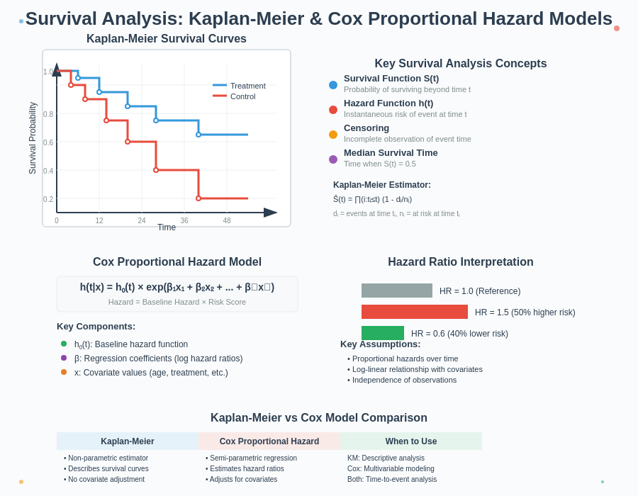
• Survival function (S(t)): Probability of surviving beyond time t
• Hazard function (h(t)): Instantaneous rate of failure at time t
• Censoring: When complete information about survival time is unavailable
• Time-to-event data: Records when subjects experience the event of interest

Why Traditional Statistical Methods Fall Short

Standard statistical techniques prove inadequate for survival data because:

Limitation	Explanation	Impact on Analysis
Censoring	Traditional methods can’t properly account for censored observations	Biased and unreliable results
Non-normality	Survival times are rarely normally distributed	Parametric assumptions violated
Time-dependent covariates	Many factors affecting survival change over time	Static models produce misleading conclusions
Unequal follow-up	Subjects enter and exit studies at different times	Simple averages distort true survival patterns

The Kaplan-Meier Method Explained

What is the Kaplan-Meier Estimator?

The Kaplan-Meier estimator (also called the product-limit estimator) provides a non-parametric estimate of the survival function from lifetime data. Developed by Edward Kaplan and Paul Meier in 1958, this method has become the gold standard for visualizing and analyzing survival data.

The Kaplan-Meier curve visually represents the probability of survival over time, accounting for censored observations. Each step in the curve corresponds to one or more events (like deaths or failures).

Calculating the Kaplan-Meier Estimate

The formula for the Kaplan-Meier estimator at time t is:

S(t) = ∏ᵢ (1 – dᵢ/nᵢ)

Where:

• dᵢ = number of events at time tᵢ
• nᵢ = number of subjects at risk at time tᵢ
• ∏ represents the product of terms for all time points where tᵢ ≤ t

Interpreting Kaplan-Meier Curves

A Kaplan-Meier curve provides several key insights:

• Median survival time: The time at which the survival probability equals 0.5
• Survival probabilities: The estimated probability of surviving beyond any specific time point
• Confidence intervals: The precision of survival estimates at various time points
• Visual comparison: When plotting multiple groups, differences in survival patterns become apparent

Testing for Differences Between Groups

When comparing survival between groups (like treatment vs. control), researchers typically use:

Test	Best Used When	Key Characteristics
Log-rank test	No crossing of survival curves	Tests overall difference between curves
Wilcoxon test	Early differences matter more	Gives more weight to early events
Peto test	Late differences matter more	Emphasizes events occurring later
Fleming-Harrington	Custom weighting needed	Allows flexible weighting of early vs. late events

The log-rank test remains the most widely used approach, calculating the observed vs. expected events in each group under the null hypothesis of no difference.

Cox Proportional Hazard Model: Beyond Simple Comparisons

What is the Cox Proportional Hazard Model?

The Cox proportional hazard model, introduced by Sir David Cox in 1972, revolutionized survival analysis by enabling examination of how multiple variables simultaneously affect survival. Unlike fully parametric approaches, Cox’s model makes no assumptions about the shape of the baseline hazard function.

The model assumes that the hazard ratio between different strata remains constant over time – the critical “proportional hazards” assumption.

The Mathematical Framework

The Cox model expresses the hazard function as:

h(t|X) = h₀(t) × exp(β₁X₁ + β₂X₂ + … + βₚXₚ)

Where:

• h₀(t) = baseline hazard function
• X₁, X₂, …, Xₚ = predictor variables
• β₁, β₂, …, βₚ = regression coefficients
• exp(βᵢXᵢ) = hazard ratio for a one-unit change in Xᵢ

Assessing Proportional Hazard Assumption

The validity of Cox model results depends on the proportional hazards assumption. Several methods test this assumption:

• Schoenfeld residual plots: Should show random patterns without time trends
• Log-minus-log plots: Parallel lines indicate proportional hazards
• Time-dependent covariates: Non-significant interaction with time supports the assumption
• Goodness-of-fit tests: Statistical tests like the Grambsch-Therneau test

Interpreting Hazard Ratios

Hazard ratios (HR) quantify the effect of predictors on survival:

• HR > 1: Increased hazard (worse survival)
• HR = 1: No effect
• HR < 1: Decreased hazard (better survival)

For example, a hazard ratio of 1.5 for a treatment means the treatment group has a 50% higher risk of experiencing the event at any given time compared to the reference group.

Practical Applications in Research

Clinical Trials and Medical Research

Survival analysis forms the backbone of many pivotal clinical studies:

• Cancer research: Comparing progression-free survival between treatments
• Cardiovascular studies: Analyzing time to cardiac events
• Drug development: Establishing efficacy based on survival benefits
• Public health interventions: Evaluating impact on mortality rates

The landmark CONCORD programme uses these methods to compare cancer survival globally, informing health policies in numerous countries.

Engineering and Reliability Analysis

Beyond medicine, survival analysis helps engineers predict:

• Component failure rates: When parts will likely fail
• System reliability: Probability of continuous operation
• Warranty planning: Optimal coverage periods
• Maintenance scheduling: When preventive maintenance maximizes uptime

Business and Customer Analytics

Companies leverage survival methods to understand:

Business Question	Survival Analysis Application
Customer churn	Time until a customer cancels a subscription
Product lifecycle	Duration until product replacement
Credit risk	Time until loan default
Employee retention	Length of employment before resignation

Kaplan-Meier vs. Cox Model Visualization

When to Use Each Method

Aspect	Kaplan-Meier	Cox Proportional Hazard
Purpose	Estimate and visualize survival	Model effect of variables on survival
Covariates	Limited to categorical groups	Multiple continuous or categorical variables
Assumptions	Non-parametric (minimal)	Proportional hazards
Output	Survival curve	Hazard ratios
Best for	Initial exploration, visualization	Multivariable analysis, effect estimation

Complementary Roles in Analysis

Most thorough survival analyses employ both approaches:

1. Begin with Kaplan-Meier curves to visualize data and identify patterns
2. Use log-rank tests to detect differences between groups
3. Apply Cox models to quantify effects while controlling for confounders
4. Check assumptions and perform sensitivity analyses

This sequential approach provides both accessible visualizations and rigorous statistical inference.

Advanced Extensions of Survival Models

Time-Dependent Covariates

Standard Cox models assume that predictor effects remain constant, but this assumption often proves unrealistic. Time-dependent covariates allow predictors to change values throughout the study period, providing more accurate models in dynamic environments.

Consider a clinical trial where treatment dosage adjusts based on patient response. A time-dependent Cox model captures these changing treatment intensities, whereas standard models would oversimplify this crucial variation.

Implementation requires specialized data formatting with:

• Multiple rows per subject
• Start and stop times for each interval
• Updated covariate values for each time segment
• Event indicators for the final interval only

Competing Risks Analysis

Competing risks arise when subjects can experience multiple, mutually exclusive event types. For instance, in cancer studies, patients might experience:

1. Cancer recurrence
2. Death from cancer
3. Death from other causes

Traditional Kaplan-Meier analysis treating non-events of interest as censored produces biased estimates. Instead, cumulative incidence functions (CIFs) properly account for competing events.

Traditional Approach	Competing Risks Approach
Treats competing events as censored	Explicitly models multiple event types
Overestimates event probability	Produces unbiased event probabilities
Assumes independence between event types	Accounts for dependencies between competing events
Single cause-specific hazard	Subdistribution hazards for each event type

The Fine and Gray model extends Cox regression for competing risks scenarios, modeling subdistribution hazards rather than cause-specific hazards.

Frailty Models for Clustered Data

When observations cluster within groups (like patients within hospitals or repeated measures within patients), frailty models address resulting correlation by introducing random effects.

Mathematically represented as:

h(t|X, Z) = h₀(t) × exp(βX + Z)

Where Z represents the frailty term (random effect) following distributions like gamma or normal.

Common applications include:

• Multi-center clinical trials
• Family-based genetic studies
• Recurrent event analysis
• Meta-analyses of survival data

Implementing Survival Analysis in Practice

Essential Software Tools

Software	Strengths	Notable Packages/Functions
R	Most comprehensive survival analysis ecosystem	survival, survminer, cmprsk
Python	Integration with machine learning workflows	lifelines, scikit-survival
SAS	Industry standard for regulated environments	PROC LIFETEST, PROC PHREG
SPSS	User-friendly interface	Kaplan-Meier, Cox Regression modules
Stata	Elegant syntax for complex models	stcox, stcurve commands

R’s survival package remains the gold standard, offering exceptional flexibility for both standard and advanced methods. The survminer package provides publication-quality visualizations of survival curves with minimal coding.

Common Pitfalls and Best Practices

Even experienced analysts encounter challenges with survival data:

• Violation of proportional hazards: Test this assumption and consider stratified models or time-dependent effects when violated
• Influential observations: Use dfbeta residuals to identify subjects exerting undue influence
• Collinearity among predictors: Check variance inflation factors and consider principal component analysis
• Overfitting: Follow the rule of thumb of at least 10 events per predictor variable
• Selection bias in cohort assembly: Clearly define entry criteria and consider inverse probability weighting

Sample Size and Power Considerations

Determining adequate sample size for survival studies requires specifying:

1. Expected event rates in each group
2. Anticipated effect size (hazard ratio)
3. Desired power (typically 80-90%)
4. Significance level (usually 0.05)
5. Accrual and follow-up periods
6. Expected dropout rate

Specialized software like PASS or the powerSurvEpi R package can calculate required sample sizes for complex survival designs.

Frequently Asked Questions